Connect your model to Nextmv with the Python SDK
⌛️ Approximate time to complete: 20 min.
In this tutorial you will learn how to bring your own decision model to the Nextmv Platform, from scratch. Complete this tutorial if you:
- Have a pre-existing decision model and you want to explore the Nextmv Platform using the Python SDK.
- Are fluent using Python 🐍.
- Are familiar using
uvfor managing Python.
To complete this tutorial, we will use two external examples, working under the principle that they are not Nextmv-created decision models. You can, and should, use your own decision model, or follow along with the examples provided:
At a high level, this tutorial will go through the following steps using both examples:
- Nextmv-ify the decision model.
- Run it locally.
- Track local runs remotely.
- Push the model to Nextmv Cloud.
- Run the model remotely.
- Perform scenario testing.
You may follow along with the full tutorial code. Let’s dive right in 🤿.
1. Prepare the executable code
Info
If you are working with your own decision model and already know that it executes, feel free to skip this step.
The decision model is composed of executable code that solves an optimization
problem. Copy the desired example code to a script named main.py.
#  ___________________________________________________________________________
#
#  Pyomo: Python Optimization Modeling Objects
#  Copyright (c) 2015-2025
#  National Technology and Engineering Solutions of Sandia, LLC
#  Under the terms of Contract DE-NA0003525 with National Technology and
#  Engineering Solutions of Sandia, LLC, the U.S. Government retains certain
#  rights in this software.
#  This software is distributed under the 3-clause BSD License.
#  ___________________________________________________________________________


#!/usr/bin/env python
# -*- coding: utf-8 -*-

# Import
from pyomo.environ import *

# Creation of a Concrete Model
model = ConcreteModel()

## Define sets ##
#  Sets
#       i   canning plants   / seattle, san-diego /
#       j   markets          / new-york, chicago, topeka / ;
model.i = Set(initialize=['seattle','san-diego'], doc='Canning plants')
model.j = Set(initialize=['new-york','chicago', 'topeka'], doc='Markets')

## Define parameters ##
#   Parameters
#       a(i)  capacity of plant i in cases
#         /    seattle     350
#              san-diego   600  /
#       b(j)  demand at market j in cases
#         /    new-york    325
#              chicago     300
#              topeka      275  / ;
model.a = Param(model.i, initialize={'seattle':350,'san-diego':600}, doc='Capacity of plant i in cases')
model.b = Param(model.j, initialize={'new-york':325,'chicago':300,'topeka':275}, doc='Demand at market j in cases')
#  Table d(i,j)  distance in thousands of miles
#                    new-york       chicago      topeka
#      seattle          2.5           1.7          1.8
#      san-diego        2.5           1.8          1.4  ;
dtab = {
    ('seattle',  'new-york') : 2.5,
    ('seattle',  'chicago')  : 1.7,
    ('seattle',  'topeka')   : 1.8,
    ('san-diego','new-york') : 2.5,
    ('san-diego','chicago')  : 1.8,
    ('san-diego','topeka')   : 1.4,
    }
model.d = Param(model.i, model.j, initialize=dtab, doc='Distance in thousands of miles')
#  Scalar f  freight in dollars per case per thousand miles  /90/ ;
model.f = Param(initialize=90, doc='Freight in dollars per case per thousand miles')
#  Parameter c(i,j)  transport cost in thousands of dollars per case ;
#            c(i,j) = f * d(i,j) / 1000 ;
def c_init(model, i, j):
  return model.f * model.d[i,j] / 1000
model.c = Param(model.i, model.j, initialize=c_init, doc='Transport cost in thousands of dollar per case')

## Define variables ##
#  Variables
#       x(i,j)  shipment quantities in cases
#       z       total transportation costs in thousands of dollars ;
#  Positive Variable x ;
model.x = Var(model.i, model.j, bounds=(0.0,None), doc='Shipment quantities in case')

## Define constraints ##
# supply(i)   observe supply limit at plant i
# supply(i) .. sum (j, x(i,j)) =l= a(i)
def supply_rule(model, i):
  return sum(model.x[i,j] for j in model.j) <= model.a[i]
model.supply = Constraint(model.i, rule=supply_rule, doc='Observe supply limit at plant i')
# demand(j)   satisfy demand at market j ;
# demand(j) .. sum(i, x(i,j)) =g= b(j);
def demand_rule(model, j):
  return sum(model.x[i,j] for i in model.i) >= model.b[j]
model.demand = Constraint(model.j, rule=demand_rule, doc='Satisfy demand at market j')

## Define Objective and solve ##
#  cost        define objective function
#  cost ..        z  =e=  sum((i,j), c(i,j)*x(i,j)) ;
#  Model transport /all/ ;
#  Solve transport using lp minimizing z ;
def objective_rule(model):
  return sum(model.c[i,j]*model.x[i,j] for i in model.i for j in model.j)
model.objective = Objective(rule=objective_rule, sense=minimize, doc='Define objective function')


## Display of the output ##
# Display x.l, x.m ;
def pyomo_postprocess(options=None, instance=None, results=None):
  model.x.display()

# This is an optional code path that allows the script to be run outside of
# pyomo command-line.  For example:  python transport.py
if __name__ == '__main__':
    # This emulates what the pyomo command-line tools does
    from pyomo.opt import SolverFactory
    import pyomo.environ
    opt = SolverFactory("glpk")
    results = opt.solve(model)
    #sends results to stdout
    results.write()
    print("\nDisplaying Solution\n" + '-'*60)
    pyomo_postprocess(None, model, results)
# Example of a shortest path network flow in a graph
# Shows integration of highspy with networkx

import highspy
import networkx as nx

orig, dest = ('A', 'D')

# create directed graph with edge weights (distances)
G = nx.DiGraph()
G.add_weighted_edges_from([('A', 'B', 2.0), ('B', 'C', 3.0), ('A', 'C', 1.5), ('B', 'D', 2.5), ('C', 'D', 1.0)])

h = highspy.Highs()
h.silent()

x = h.addBinaries(G.edges, obj=nx.get_edge_attributes(G, 'weight'))

# add flow conservation constraints
#                        {  1  if n = orig
#   sum(out) - sum(in) = { -1  if n = dest
#                        {  0     otherwise
rhs  = lambda n: 1 if n == orig else -1 if n == dest else 0
flow = lambda E: h.qsum((x[e] for e in E))

h.addConstrs(flow(G.out_edges(n)) - flow(G.in_edges(n)) == rhs(n) for n in G.nodes)
h.minimize()

# Print the solution
print('Shortest path from', orig, 'to', dest, 'is: ', end = '')
sol = h.vals(x)

n = orig
while n != dest:
    print(n, end=' ')
    n = next(e[1] for e in G.out_edges(n) if sol[e] > 0.5)

print(dest)
2. Install requirements
Info
If you are working with your own decision model and already have all requirements ready for it, feel free to skip this step.
If you are following along with the full tutorial code,
you should be using the original directory. In that case, run the following
command in the root of your project.
On the other hand, if you are completing this tutorial from scratch, run the following command in the root of your project.
The Pyomo example uses the GLPK solver. Make sure you install it as well.
For Windows, install from SourceForge.
3. Run the executable code
Info
If you are working with your own decision model and already know that it executes, feel free to skip this step.
Make sure your decision model works by running the executable code.
# ==========================================================
# = Solver Results                                         =
# ==========================================================
# ----------------------------------------------------------
#   Problem Information
# ----------------------------------------------------------
Problem:
- Name: unknown
  Lower bound: 153.675
  Upper bound: 153.675
  Number of objectives: 1
  Number of constraints: 5
  Number of variables: 6
  Number of nonzeros: 12
  Sense: minimize
# ----------------------------------------------------------
#   Solver Information
# ----------------------------------------------------------
Solver:
- Status: ok
  Termination condition: optimal
  Statistics:
    Branch and bound:
      Number of bounded subproblems: 0
      Number of created subproblems: 0
  Error rc: 0
  Time: 0.006303071975708008
# ----------------------------------------------------------
#   Solution Information
# ----------------------------------------------------------
Solution:
- number of solutions: 0
  number of solutions displayed: 0

Displaying Solution
------------------------------------------------------------
x : Shipment quantities in case
    Size=6, Index=i*j
    Key                       : Lower : Value : Upper : Fixed : Stale : Domain
    ('san-diego', 'chicago') :   0.0 :   0.0 :  None : False : False :  Reals
    ('san-diego', 'new-york') :   0.0 : 275.0 :  None : False : False :  Reals
      ('san-diego', 'topeka') :   0.0 : 275.0 :  None : False : False :  Reals
      ('seattle', 'chicago') :   0.0 : 300.0 :  None : False : False :  Reals
      ('seattle', 'new-york') :   0.0 :  50.0 :  None : False : False :  Reals
        ('seattle', 'topeka') :   0.0 :   0.0 :  None : False : False :  Reals
4. Nextmv-ify the decision model
We are going to turn the executable decision model into a Nextmv application.
Tip
Go to the Applications section to learn more about Nextmv applications.
We are going to adapt the examples so that they can follow the conventions of a Nextmv application, such as:
- The app receives one, or more, inputs (problem data) through
stdinor files. - The app run can be configured through options that are received as CLI arguments.
- The app processes the inputs, and executes the decision model.
- The app produces one, or more, outputs (solutions) and prints to
stdoutor files. - The app optionally produces metrics and assets (can be visual, like charts).
Start by adding the app.yaml file, which is known as the app
manifest, to the root of the project. This file contains the
configuration of the app.
type: python
runtime: ghcr.io/nextmv-io/runtime/pyomo:latest
files:
  - main.py
python:
  pip-requirements: pyproject.toml # Can be a requirements.txt
configuration:
  content:
    format: json
  options:
    items:
      - name: duration
        description: Duration for the solver, in seconds.
        required: false
        option_type: int
        default: 1
        additional_attributes:
          min: 0
          max: 10
          step: 1
        ui:
          control_type: slider
      - name: solver
        description: Solver provider to use.
        required: false
        option_type: string
        default: glpk
        additional_attributes:
          values:
            - scip
            - cbc
            - glpk
        ui:
          control_type: select
type: python
runtime: ghcr.io/nextmv-io/runtime/python:3.11
files:
  - main.py
python:
  pip-requirements: pyproject.toml # Can be a requirements.txt
configuration:
  content:
    format: multi-file
    multi-file:
      input:
        path: inputs
      output:
        solutions: outputs/solutions
        metrics: outputs/metrics.json
        assets: outputs/assets.json
  options:
    items:
      - name: duration
        description: Duration for the solver, in seconds.
        required: false
        option_type: float
        default: 1
        additional_attributes:
          min: 0
          max: 10
          step: 1
        ui:
          control_type: slider
This tutorial is not meant to discuss the app manifest in-depth, for that you can go to the manifest docs. However, these are the main attributes shown in the manifests:
type: both arepythonapplications.runtime: Pyomo uses the specialpyomo:latestruntime, as it comes with solvers pre-installed. HiGHS uses the standardpython:3.11runtime.files: contains files that make up the executable code of the app. In both cases only a singlemain.pyfile is needed. Make sure to include all files and dirs that are needed for your decision model.python.pip-requirements: specifies in both cases the file with the Python packages that need to be installed for the application.configuration.content: Pyomo will use thejsonformat, so it does not need additional configurations. HiGHS will usemulti-file, so additional configurations are needed. As you complete this tutorial, the difference between the two formats will become clearer.configuration.options: for both examples, we are adding options to the application, which allow you to configure runs, with parameters such as solver duration.
For both examples, a dependency for nextmv (the Nextmv Python
SDK) is also added. This dependency is optional, and SDK
modeling constructs are not needed to run a Nextmv
Application. However, using the SDK modeling features makes it easier to work
with Nextmv apps, as a lot of convenient functionality is already baked in.
Run the following command to add the nextmv dependency to your project.
Now, you can overwrite your main.py files with the Nextmv-ified version.
#  ___________________________________________________________________________
#
#  Pyomo: Python Optimization Modeling Objects
#  Copyright (c) 2015-2025
#  National Technology and Engineering Solutions of Sandia, LLC
#  Under the terms of Contract DE-NA0003525 with National Technology and
#  Engineering Solutions of Sandia, LLC, the U.S. Government retains certain
#  rights in this software.
#  This software is distributed under the 3-clause BSD License.
#  ___________________________________________________________________________


#!/usr/bin/env python
# -*- coding: utf-8 -*-


import nextmv

# Import
from pyomo.environ import *

# Duration parameter for the solver.
SUPPORTED_PROVIDER_DURATIONS = {
    "cbc": "sec",
    "glpk": "tmlim",
    "scip": "limits/time",
}

# Creation of a Concrete Model
model = ConcreteModel()

nextmv.redirect_stdout()
input = nextmv.load()
options = input.options

## Define sets ##
#  Sets
#       i   canning plants   / seattle, san-diego /
#       j   markets          / new-york, chicago, topeka / ;
sets = input.data["sets"]
model.i = Set(initialize=sets["i"], doc="Canning plants")
model.j = Set(initialize=sets["j"], doc="Markets")

## Define parameters ##
#   Parameters
#       a(i)  capacity of plant i in cases
#         /    seattle     350
#              san-diego   600  /
#       b(j)  demand at market j in cases
#         /    new-york    325
#              chicago     300
#              topeka      275  / ;
params = input.data["parameters"]
model.a = Param(
    model.i,
    initialize=params["a"],
    doc="Capacity of plant i in cases",
)
model.b = Param(
    model.j,
    initialize=params["b"],
    doc="Demand at market j in cases",
)
#  Table d(i,j)  distance in thousands of miles
#                    new-york       chicago      topeka
#      seattle          2.5           1.7          1.8
#      san-diego        2.5           1.8          1.4  ;
dtab = {(edge["from"], edge["to"]): edge["cost"] for edge in params["d"]}
model.d = Param(model.i, model.j, initialize=dtab, doc="Distance in thousands of miles")
#  Scalar f  freight in dollars per case per thousand miles  /90/ ;
model.f = Param(
    initialize=params["f"], doc="Freight in dollars per case per thousand miles"
)


#  Parameter c(i,j)  transport cost in thousands of dollars per case ;
#            c(i,j) = f * d(i,j) / 1000 ;
def c_init(model, i, j):
    return model.f * model.d[i, j] / 1000


model.c = Param(
    model.i,
    model.j,
    initialize=c_init,
    doc="Transport cost in thousands of dollar per case",
)

## Define variables ##
#  Variables
#       x(i,j)  shipment quantities in cases
#       z       total transportation costs in thousands of dollars ;
#  Positive Variable x ;
model.x = Var(model.i, model.j, bounds=(0.0, None), doc="Shipment quantities in case")


## Define constraints ##
# supply(i)   observe supply limit at plant i
# supply(i) .. sum (j, x(i,j)) =l= a(i)
def supply_rule(model, i):
    return sum(model.x[i, j] for j in model.j) <= model.a[i]


model.supply = Constraint(
    model.i, rule=supply_rule, doc="Observe supply limit at plant i"
)


# demand(j)   satisfy demand at market j ;
# demand(j) .. sum(i, x(i,j)) =g= b(j);
def demand_rule(model, j):
    return sum(model.x[i, j] for i in model.i) >= model.b[j]


model.demand = Constraint(model.j, rule=demand_rule, doc="Satisfy demand at market j")


## Define Objective and solve ##
#  cost        define objective function
#  cost ..        z  =e=  sum((i,j), c(i,j)*x(i,j)) ;
#  Model transport /all/ ;
#  Solve transport using lp minimizing z ;
def objective_rule(model):
    return sum(model.c[i, j] * model.x[i, j] for i in model.i for j in model.j)


model.objective = Objective(
    rule=objective_rule, sense=minimize, doc="Define objective function"
)


## Display of the output ##
# Display x.l, x.m ;
def pyomo_postprocess(options=None, instance=None, results=None):
    model.x.display()


# This is an optional code path that allows the script to be run outside of
# pyomo command-line.  For example:  python transport.py
if __name__ == "__main__":
    # This emulates what the pyomo command-line tools does
    from pyomo.opt import SolverFactory

    opt = SolverFactory(options.solver)
    opt.options[SUPPORTED_PROVIDER_DURATIONS[options.solver]] = options.duration
    results = opt.solve(model)
    # sends results to stdout
    results.write()
    print("\nDisplaying Solution\n" + "-" * 60)
    pyomo_postprocess(None, model, results)

    shipments = [
        {"from": ix[0], "to": ix[1], "quantity": x()}
        for ix, x in model.x.items()
        if x() > 0.01
    ]
    solution = {"shipments": shipments}
    metrics = {
        "duration": results.solver.time,
        "value": value(model.objective, exception=False),
        "variables": model.nvariables(),
        "constraints": model.nconstraints(),
        "num_edges_used": len(shipments),
    }
    nextmv.write(solution=solution, metrics=metrics)
# Example of a shortest path network flow in a graph
# Shows integration of highspy with networkx

import highspy
import networkx as nx
import nextmv

nextmv.redirect_stdout()
input = nextmv.load(
    data_files=[
        nextmv.json_data_file("nodes", input_data_key="nodes"),
        nextmv.csv_data_file("edges", input_data_key="edges"),
    ],
)
options = input.options

nodes = input.data["nodes"]
orig, dest = (nodes["origin"], nodes["destination"])

# create directed graph with edge weights (distances)
G = nx.DiGraph()
G.add_weighted_edges_from(
    [(edge["from"], edge["to"], float(edge["weight"])) for edge in input.data["edges"]]
)

h = highspy.Highs()
h.setOptionValue("time_limit", options.duration)

x = h.addBinaries(G.edges, obj=nx.get_edge_attributes(G, "weight"))

# add flow conservation constraints
#                        {  1  if n = orig
#   sum(out) - sum(in) = { -1  if n = dest
#                        {  0     otherwise
rhs = lambda n: 1 if n == orig else -1 if n == dest else 0
flow = lambda E: h.qsum((x[e] for e in E))

h.addConstrs(flow(G.out_edges(n)) - flow(G.in_edges(n)) == rhs(n) for n in G.nodes)
h.minimize()

# Print the solution
shortest_path = []
print("Shortest path from", orig, "to", dest, "is: ", end="")
sol = h.vals(x)

n = orig
while n != dest:
    shortest_path.append(n)
    print(n, end=" ")
    n = next(e[1] for e in G.out_edges(n) if sol[e] > 0.5)

print(dest)

solution = {"shortest_path": shortest_path}
metrics = {
    "duration": h.getRunTime(),
    "value": h.getInfo().objective_function_value,
    "variables": h.numVariables,
    "constraints": h.numConstrs,
    "length_shortest_path": len(shortest_path),
}
nextmv.write(
    options=options,
    metrics=metrics,
    solution_files=[
        nextmv.json_solution_file(name="shortest_path", data=solution),
    ],
)
This is a short summary of the changes introduced for each of the examples:
- Read the
app.yamlfile and its configurations. - The input data is no longer in the Python file itself. We will move it to a
file under
inputs/problem.json. In a singlejsonfile we will define the complete input. Given that we are working with thejsoncontent format, we use the Python SDK to load the input data fromstdin. - Modify the definition of sets, and parameters to use the data from the loaded input.
- Store the solution to the problem, and solver metrics (statistics), in an output.
- Write the output to
stdout, given that we are working with thejsoncontent format.
- Read the
app.yamlfile and its configurations. - The input data is no longer in the Python file itself. We are representing
the problem with several files under the
inputsdirectory. Ininputs/edges.csvwe are going to write the edges with their corresponding weights. Ininputs/nodes.jsonwe are going to set the information about nodes, like which node is the origin and which is the destination. When working with more than one file, themulti-filecontent format is ideal. We use the Python SDK to load the input data from the various files. - Modify the definition of nodes, edges, and decision variables to use data from the loaded inputs.
- Store the solution to the problem, and solver metrics (statistics), in an output.
- Write the output to several files, under the
outputsdirectory, given that we are working with themulti-filecontent format.
Place the following data files in an inputs directory.
{
  "sets": {
    "i": ["seattle", "san-diego"],
    "j": ["new-york", "chicago", "topeka"]
  },
  "parameters": {
    "a": {
      "seattle": 350,
      "san-diego": 600
    },
    "b": {
      "new-york": 325,
      "chicago": 300,
      "topeka": 275
    },
    "d": [
      { "from": "seattle", "to": "new-york", "cost": 2.5 },
      { "from": "seattle", "to": "chicago", "cost": 1.7 },
      { "from": "seattle", "to": "topeka", "cost": 1.8 },
      { "from": "san-diego", "to": "new-york", "cost": 2.5 },
      { "from": "san-diego", "to": "chicago", "cost": 1.8 },
      { "from": "san-diego", "to": "topeka", "cost": 1.4 }
    ],
    "f": 90
  }
}
After you are done Nextmv-ifying, your Nextmv app should have the following structure, for the examples provided.
Please note that even if you are not using the Python SDK's modeling constructs as part of your executable code, you still need to install it for this tutorial. On the other hand, if you decided that you want to use the Python SDK for the executable code, you would have needed to install it.
Now you are ready to explore the Nextmv Platform 🥳.
5. Run the Nextmv application locally
The local package of the Nextmv Python SDK provides
functionality to run Nextmv applications locally on your machine.
Tip
The local experience is completely free of charge and does not require a
Nextmv account.
Tip
Instead of using Python scripts, you can also use the Nextmv CLI to run applications locally. You can check out the local experience tutorial to learn more.
Create a script named app1.py, or use a cell of a Jupyter notebook. Copy and
paste the following code into it, making sure you use the correct app src
(for this example, the current working directory, ".").:
import os
import time

import nextmv
from nextmv import local

# Instantiate the local application.
local_app = local.Application(src=".")

# Provide any input you want for the app. This input can come from a file, for
# example.
problem = nextmv.load(path=os.path.join("inputs", "problem.json"))
run_id_1 = local_app.new_run(input=problem.data)

# Sleep and get metadata, output (results), logs.
time.sleep(5)

run_information_1 = local_app.run_information(run_id=run_id_1)
nextmv.write(run_information_1)

run_results_1 = local_app.run_result(run_id=run_id_1)
nextmv.write(run_results_1.output)

run_logs_1 = local_app.run_logs(run_id=run_id_1)
print(run_logs_1)
import time

import nextmv
from nextmv import local

# Instantiate the local application.
local_app = local.Application(src=".")

# Provide any input you want for the app. This input can come from a file, for
# example.
run_id_1 = local_app.new_run(input_dir_path="./inputs")

# Sleep and get metadata, output (results), logs.
time.sleep(5)

run_information_1 = local_app.run_information(run_id=run_id_1)
nextmv.write(run_information_1)

run_results_1 = local_app.run_result(run_id=run_id_1, output_dir_path="./outputs")

run_logs_1 = local_app.run_logs(run_id=run_id_1)
print(run_logs_1)
When you instantiate a local application, the src argument must point to a
directory where the app.yaml manifest file is located.
This will print the IDs of the runs created. The app runs start in the background. Run the script, or notebook cell, to get an output similar to this:
{
  "description": "Local run created at 2025-11-10T17:20:43.386461Z",
  "id": "local-h61b3nvr",
  "metadata": {
    "application_id": ".",
    "application_instance_id": "",
    "application_version_id": "",
    "created_at": "2025-11-10T17:20:43.386461Z",
    "duration": 1063.7,
    "error": "",
    "input_size": 877.0,
    "output_size": 0.0,
    "format": {
      "input": {
        "type": "json"
      },
      "output": {
        "type": "json"
      }
    },
    "status_v2": "succeeded"
  },
  "name": "local run local-h61b3nvr",
  "user_email": "",
  "console_url": ""
}
{
  "options": {
    "duration": 1,
    "solver": "glpk",
    "input": "",
    "output": ""
  },
  "solution": {
    "shipments": [
      {
        "from": "seattle",
        "to": "new-york",
        "quantity": 50.0
      },
      {
        "from": "seattle",
        "to": "chicago",
        "quantity": 300.0
      },
      {
        "from": "san-diego",
        "to": "new-york",
        "quantity": 275.0
      },
      {
        "from": "san-diego",
        "to": "topeka",
        "quantity": 275.0
      }
    ]
  },
  "statistics": {
    "result": {
      "duration": 0.006533145904541016,
      "value": 153.67499999999998,
      "custom": {
        "variables": 6,
        "constraints": 5,
        "num_edges_used": 4
      }
    },
    "schema": "v1"
  },
  "assets": []
}
# ==========================================================
# = Solver Results                                         =
# ==========================================================
# ----------------------------------------------------------
#   Problem Information
# ----------------------------------------------------------
Problem:
- Name: unknown
  Lower bound: 153.675
  Upper bound: 153.675
  Number of objectives: 1
  Number of constraints: 5
  Number of variables: 6
  Number of nonzeros: 12
  Sense: minimize
# ----------------------------------------------------------
#   Solver Information
# ----------------------------------------------------------
Solver:
- Status: ok
  Termination condition: optimal
  Statistics:
    Branch and bound:
      Number of bounded subproblems: 0
      Number of created subproblems: 0
  Error rc: 0
  Time: 0.006533145904541016
# ----------------------------------------------------------
#   Solution Information
# ----------------------------------------------------------
Solution:
- number of solutions: 0
  number of solutions displayed: 0

Displaying Solution
------------------------------------------------------------
x : Shipment quantities in case
    Size=6, Index=i*j
    Key                       : Lower : Value : Upper : Fixed : Stale : Domain
    ('san-diego', 'chicago') :   0.0 :   0.0 :  None : False : False :  Reals
    ('san-diego', 'new-york') :   0.0 : 275.0 :  None : False : False :  Reals
      ('san-diego', 'topeka') :   0.0 : 275.0 :  None : False : False :  Reals
      ('seattle', 'chicago') :   0.0 : 300.0 :  None : False : False :  Reals
      ('seattle', 'new-york') :   0.0 :  50.0 :  None : False : False :  Reals
        ('seattle', 'topeka') :   0.0 :   0.0 :  None : False : False :  Reals
{
  "description": "Local run created at 2025-11-10T17:21:11.745145Z",
  "id": "local-pi6fotk7",
  "metadata": {
    "application_id": ".",
    "application_instance_id": "",
    "application_version_id": "",
    "created_at": "2025-11-10T17:21:11.745145Z",
    "duration": 992.9,
    "error": "",
    "input_size": 97.0,
    "output_size": 0.0,
    "format": {
      "input": {
        "type": "multi-file"
      },
      "output": {
        "type": "multi-file"
      }
    },
    "status_v2": "succeeded"
  },
  "name": "local run local-pi6fotk7",
  "user_email": "",
  "console_url": ""
}
Running HiGHS 1.12.0 (git hash: 755a8e0): Copyright (c) 2025 HiGHS under MIT licence terms
MIP has 4 rows; 5 cols; 10 nonzeros; 5 integer variables (5 binary)
Coefficient ranges:
  Matrix  [1e+00, 1e+00]
  Cost    [1e+00, 3e+00]
  Bound   [1e+00, 1e+00]
  RHS     [1e+00, 1e+00]
Presolving model
2 rows, 3 cols, 6 nonzeros  0s
0 rows, 1 cols, 0 nonzeros  0s
0 rows, 0 cols, 0 nonzeros  0s
Presolve reductions: rows 0(-4); columns 0(-5); nonzeros 0(-10) - Reduced to empty
Presolve: Optimal

Src: B => Branching; C => Central rounding; F => Feasibility pump; H => Heuristic;
    I => Shifting; J => Feasibility jump; L => Sub-MIP; P => Empty MIP; R => Randomized rounding;
    S => Solve LP; T => Evaluate node; U => Unbounded; X => User solution; Y => HiGHS solution;
    Z => ZI Round; l => Trivial lower; p => Trivial point; u => Trivial upper; z => Trivial zero

        Nodes      |    B&B Tree     |            Objective Bounds              |  Dynamic Constraints |       Work
Src  Proc. InQueue |  Leaves   Expl. | BestBound       BestSol              Gap |   Cuts   InLp Confl. | LpIters     Time

        0       0         0   0.00%   2.5             2.5                0.00%        0      0      0         0     0.0s

Solving report
  Status            Optimal
  Primal bound      2.5
  Dual bound        2.5
  Gap               0% (tolerance: 0.01%)
  P-D integral      0
  Solution status   feasible
                    2.5 (objective)
                    0 (bound viol.)
                    0 (int. viol.)
                    0 (row viol.)
  Timing            0.00
  Max sub-MIP depth 0
  Nodes             0
  Repair LPs        0
  LP iterations     0

Shortest path from A to D is: A C D
The local package allows you to perform runs on the application and store the
inputs, options, logs, and outputs that are associated with the run. As you can
tell, depending on the content format used for each application, you work with
the data differently.
- For a
jsonapplication, you send adictto thenew_runmethod. - For a
multi-fileapplication, you specify a dir where the input files are stored.
Similarly, the content format dictates how to get the output data.
- For a
jsonapplication, the outputdictcan be obtained from the results. - For a
multi-fileapplication, the output files are written to the path specified in the argument.
The run is started and completed in a background process. Instead of sleeping and waiting for the results, you can poll for the run to be finished.
Create another script, which you can name app2.py, or use another cell in the
Jupyter notebook. Copy and paste the following code into it, making sure you
use the correct app src:
import os

import nextmv
from nextmv import local

# Instantiate the local application.
local_app = local.Application(src=".")

# Start a new run, loading the data from a file, and poll for results.
problem = nextmv.load(path=os.path.join("inputs", "problem.json"))
run_results_2 = local_app.new_run_with_result(input=problem.data)
nextmv.write(run_results_2)  # This time, print both metadata and output at once.

run_logs_2 = local_app.run_logs(run_id=run_results_2.id)
print(run_logs_2)
import nextmv
from nextmv import local

# Instantiate the local application.
local_app = local.Application(src=".")

# Start a new run, loading the file from a directory, and poll for results.
run_results_2 = local_app.new_run_with_result(
    input_dir_path="./inputs",
    output_dir_path="./outputs",
)
nextmv.write(run_results_2)  # This time, print both metadata and output at once.

run_logs_2 = local_app.run_logs(run_id=run_results_2.id)
print(run_logs_2)
Running the app2.py script (or the new notebook cell), you'll notice that the
results are duplicated, as you are performing the same run but waiting for the
results concurrently.
{
  "description": "Local run created at 2025-11-17T21:44:29.206722Z",
  "id": "local-20dxditm",
  "metadata": {
    "application_id": ".",
    "application_instance_id": "",
    "application_version_id": "",
    "created_at": "2025-11-17T21:44:29.206722Z",
    "duration": 1160.7,
    "error": "",
    "input_size": 877.0,
    "output_size": 0.0,
    "format": {
      "input": {
        "type": "json"
      },
      "output": {
        "type": "json"
      }
    },
    "status_v2": "succeeded"
  },
  "name": "local run local-20dxditm",
  "user_email": "",
  "console_url": "",
  "output": {
    "options": {
      "duration": 1,
      "solver": "glpk",
      "input": "",
      "output": ""
    },
    "solution": {
      "shipments": [
        {
          "from": "seattle",
          "to": "new-york",
          "quantity": 50.0
        },
        {
          "from": "seattle",
          "to": "chicago",
          "quantity": 300.0
        },
        {
          "from": "san-diego",
          "to": "new-york",
          "quantity": 275.0
        },
        {
          "from": "san-diego",
          "to": "topeka",
          "quantity": 275.0
        }
      ]
    },
    "statistics": {
      "result": {
        "duration": 0.007156848907470703,
        "value": 153.67499999999998,
        "custom": {
          "variables": 6,
          "constraints": 5,
          "num_edges_used": 4
        }
      },
      "schema": "v1"
    },
    "assets": []
  }
}
# ==========================================================
# = Solver Results                                         =
# ==========================================================
# ----------------------------------------------------------
#   Problem Information
# ----------------------------------------------------------
Problem:
- Name: unknown
  Lower bound: 153.675
  Upper bound: 153.675
  Number of objectives: 1
  Number of constraints: 5
  Number of variables: 6
  Number of nonzeros: 12
  Sense: minimize
# ----------------------------------------------------------
#   Solver Information
# ----------------------------------------------------------
Solver:
- Status: ok
  Termination condition: optimal
  Statistics:
    Branch and bound:
      Number of bounded subproblems: 0
      Number of created subproblems: 0
  Error rc: 0
  Time: 0.007156848907470703
# ----------------------------------------------------------
#   Solution Information
# ----------------------------------------------------------
Solution:
- number of solutions: 0
  number of solutions displayed: 0

Displaying Solution
------------------------------------------------------------
x : Shipment quantities in case
    Size=6, Index=i*j
    Key                       : Lower : Value : Upper : Fixed : Stale : Domain
    ('san-diego', 'chicago') :   0.0 :   0.0 :  None : False : False :  Reals
    ('san-diego', 'new-york') :   0.0 : 275.0 :  None : False : False :  Reals
      ('san-diego', 'topeka') :   0.0 : 275.0 :  None : False : False :  Reals
      ('seattle', 'chicago') :   0.0 : 300.0 :  None : False : False :  Reals
      ('seattle', 'new-york') :   0.0 :  50.0 :  None : False : False :  Reals
        ('seattle', 'topeka') :   0.0 :   0.0 :  None : False : False :  Reals
{
  "description": "Local run created at 2025-11-17T21:44:53.418837Z",
  "id": "local-4d4fjolz",
  "metadata": {
    "application_id": ".",
    "application_instance_id": "",
    "application_version_id": "",
    "created_at": "2025-11-17T21:44:53.418837Z",
    "duration": 1073.4,
    "error": "",
    "input_size": 97.0,
    "output_size": 0.0,
    "format": {
      "input": {
        "type": "multi-file"
      },
      "output": {
        "type": "multi-file"
      }
    },
    "status_v2": "succeeded"
  },
  "name": "local run local-4d4fjolz",
  "user_email": "",
  "console_url": ""
}
Running HiGHS 1.12.0 (git hash: 755a8e0): Copyright (c) 2025 HiGHS under MIT licence terms
MIP has 4 rows; 5 cols; 10 nonzeros; 5 integer variables (5 binary)
Coefficient ranges:
  Matrix  [1e+00, 1e+00]
  Cost    [1e+00, 3e+00]
  Bound   [1e+00, 1e+00]
  RHS     [1e+00, 1e+00]
Presolving model
2 rows, 3 cols, 6 nonzeros  0s
0 rows, 1 cols, 0 nonzeros  0s
0 rows, 0 cols, 0 nonzeros  0s
Presolve reductions: rows 0(-4); columns 0(-5); nonzeros 0(-10) - Reduced to empty
Presolve: Optimal

Src: B => Branching; C => Central rounding; F => Feasibility pump; H => Heuristic;
    I => Shifting; J => Feasibility jump; L => Sub-MIP; P => Empty MIP; R => Randomized rounding;
    S => Solve LP; T => Evaluate node; U => Unbounded; X => User solution; Y => HiGHS solution;
    Z => ZI Round; l => Trivial lower; p => Trivial point; u => Trivial upper; z => Trivial zero

        Nodes      |    B&B Tree     |            Objective Bounds              |  Dynamic Constraints |       Work
Src  Proc. InQueue |  Leaves   Expl. | BestBound       BestSol              Gap |   Cuts   InLp Confl. | LpIters     Time

        0       0         0   0.00%   2.5             2.5                0.00%        0      0      0         0     0.0s

Solving report
  Status            Optimal
  Primal bound      2.5
  Dual bound        2.5
  Gap               0% (tolerance: 0.01%)
  P-D integral      0
  Solution status   feasible
                    2.5 (objective)
                    0 (bound viol.)
                    0 (int. viol.)
                    0 (row viol.)
  Timing            0.00
  Max sub-MIP depth 0
  Nodes             0
  Repair LPs        0
  LP iterations     0

Shortest path from A to D is: A C D
If you inspect the file structure of your application, you will find a tree similar to this:
.
├── .nextmv
│   └── runs
│       ├── {RUN_ID_1}
│       │   ├── inputs
│       │   │   └── input.json
│       │   ├── {RUN_ID_1}.json
│       │   ├── logs
│       │   │   └── logs.log
│       │   ├── outputs
│       │   │   ├── assets.json
│       │   │   ├── metrics.json
│       │   │   └── solutions
│       │   │       └── solution.json
│       │   └── visuals
│       └── {RUN_ID_2}
│           ├── inputs
│           │   └── input.json
│           ├── {RUN_ID_2}.json
│           ├── logs
│           │   └── logs.log
│           ├── outputs
│           │   ├── assets.json
│           │   ├── metrics.json
│           │   └── solutions
│           │       └── solution.json
│           └── visuals
├── app1.py
├── app2.py
├── app.yaml
├── inputs
│   └── problem.json
├── main.py
├── pyproject.toml
└── uv.lock
.
├── .nextmv
│   └── runs
│       ├── {RUN_ID_1}
│       │   ├── inputs
│       │   │   ├── edges.csv
│       │   │   └── nodes.json
│       │   ├── {RUN_ID_1}.json
│       │   ├── logs
│       │   │   └── logs.log
│       │   ├── outputs
│       │   │   ├── assets.json
│       │   │   ├── metrics.json
│       │   │   └── solutions
│       │   │       └── shortest_path.json
│       │   └── visuals
│       └── {RUN_ID_2}
│           ├── inputs
│           │   ├── edges.csv
│           │   └── nodes.json
│           ├── {RUN_ID_2}.json
│           ├── logs
│           │   └── logs.log
│           ├── outputs
│           │   ├── assets.json
│           │   ├── metrics.json
│           │   └── solutions
│           │       └── shortest_path.json
│           └── visuals
├── app1.py
├── app2.py
├── app.yaml
├── inputs
│   ├── edges.csv
│   └── nodes.json
├── main.py
├── outputs
│   └── shortest_path.json
├── pyproject.toml
└── uv.lock
The .nextmv dir is used to store and manage the local applications run in a
structured way. The local package is used to interact with these files, with
methods for starting runs, retrieving results, visualizing charts, and more.
6. Create an account
The local experience is a great free starting point, but the full suite of
benefits starts with a Nextmv Cloud account.
- Visit the Nextmv Console to sign up for an account at https://cloud.nextmv.io.
- Fill out the form. A member of the Nextmv team will reach out to you to complete the sign-up process.
- Log in to your account. The Nextmv Console is ready to use!
Once you have logged in to your account, you need to fetch your API key. You can do so from your settings.
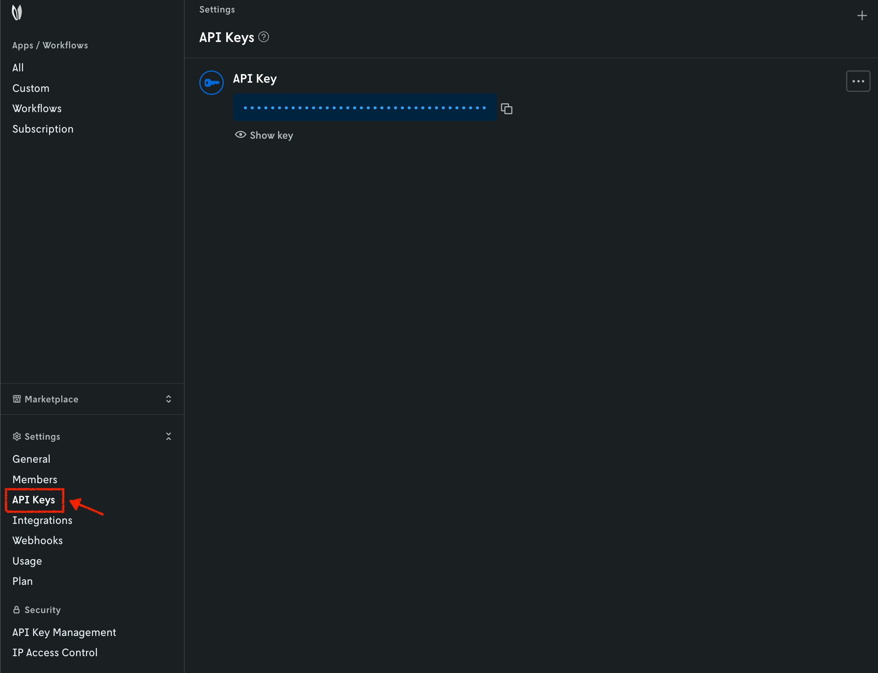
When you have your API key, it is convenient to save it as an environment variable so that you can use it for the rest of this tutorial.
7. Create a Nextmv Cloud application
Create another script, which you can name app3.py, or use another cell in the
Jupyter notebook. Copy and paste the following code into it:
After you run the script, or notebook cell, you should see an output similar to this one, where it confirms that the app was created successfully.
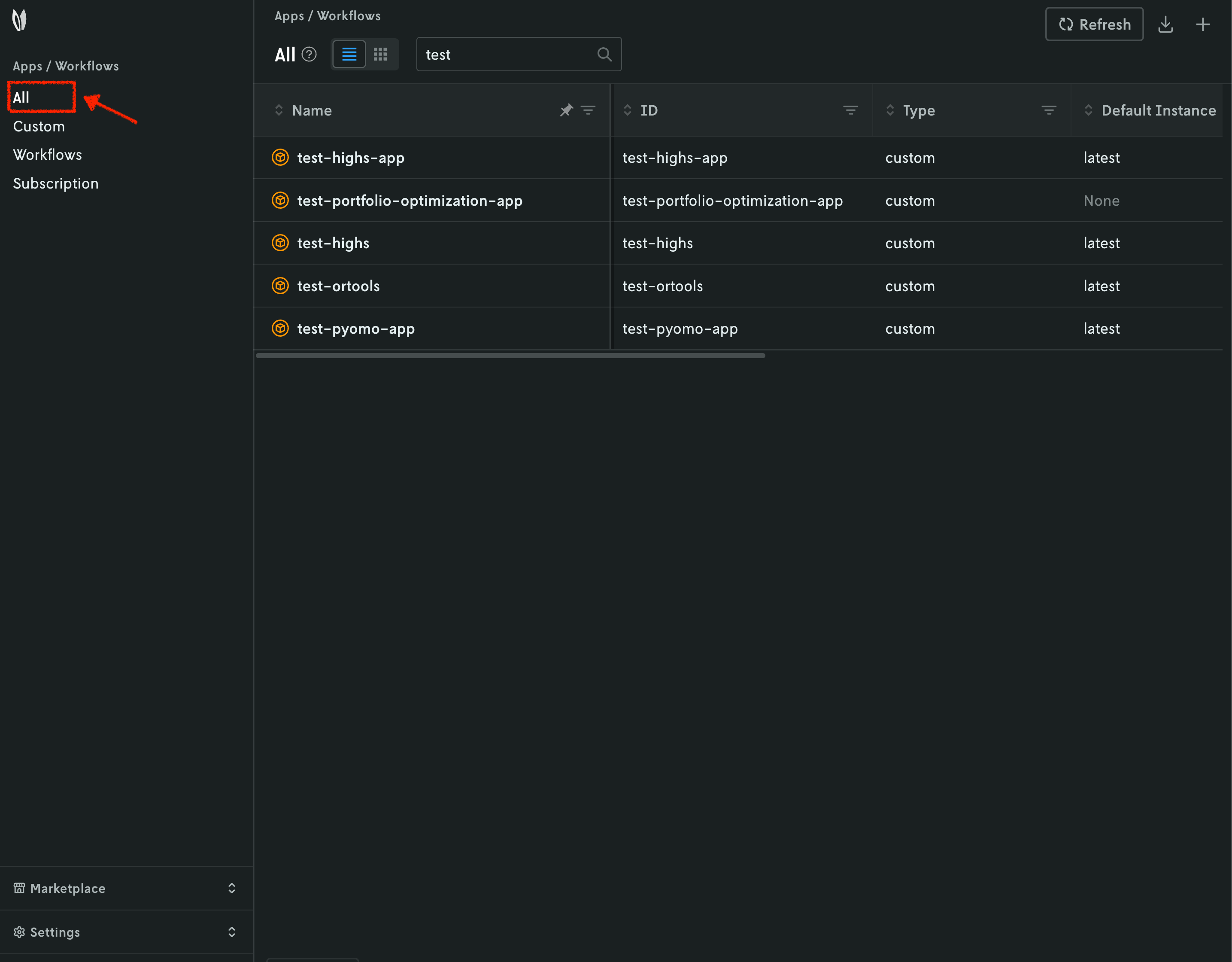
You can go to the Apps section in the Nextmv Console where you will see your applications.
8. Sync local runs to Nextmv Cloud
Create another script, which you can name app4.py, or use another cell in the
Jupyter notebook. Copy and paste the following code into it, making sure you
use the correct app src:
import os

from nextmv import cloud, local

# Instantiate the local application.
local_app = local.Application(src=".")

# Instantiate the cloud application.
client = cloud.Client(api_key=os.getenv("NEXTMV_API_KEY"))
cloud_app = cloud.Application(client=client, id="test-pyomo-app")

# Sync the local app's runs to the cloud app.
local_app.sync(target=cloud_app, verbose=True)
import os

from nextmv import cloud, local

# Instantiate the local application.
local_app = local.Application(src=".")

# Instantiate the cloud application.
client = cloud.Client(api_key=os.getenv("NEXTMV_API_KEY"))
cloud_app = cloud.Application(client=client, id="test-highs-app")

# Sync the local app's runs to the cloud app.
local_app.sync(target=cloud_app, verbose=True)
You will now track these runs in Nextmv Cloud, as external runs. After you run the script, or notebook cell, you should see an output similar to this one, where it shows which runs were synced successfully.
☁️ Starting sync of local application `.` to Nextmv Cloud application `test-highs-app`.
ℹ️  Found 4 local runs to sync from ./.nextmv/runs.
🔄 Syncing local run `local-gmrkwzrp`...
✅ Synced local run `local-gmrkwzrp` as remote run `{'run_id': 'latest-uPu85_zDg', 'synced_at': '2025-11-10T19:40:00.130408Z', 'app_id': 'test-highs-app'}`.
🔄 Syncing local run `local-ihnmua49`...
✅ Synced local run `local-ihnmua49` as remote run `{'run_id': 'latest-P5RwclkDg', 'synced_at': '2025-11-10T19:40:04.842384Z', 'app_id': 'test-highs-app'}`.
🔄 Syncing local run `local-v8wh5r82`...
✅ Synced local run `local-v8wh5r82` as remote run `{'run_id': 'latest-zRnwclzvg', 'synced_at': '2025-11-10T19:40:09.561436Z', 'app_id': 'test-highs-app'}`.
🔄 Syncing local run `local-suoz75x3`...
✅ Synced local run `local-suoz75x3` as remote run `{'run_id': 'latest-i8DQ5_kDg', 'synced_at': '2025-11-10T19:40:14.467164Z', 'app_id': 'test-highs-app'}`.
🚀 Process completed, synced local application `.` to Nextmv Cloud application `test-highs-app`: 4/4 runs.
Depending on the number of times you run the script, you might be syncing more or fewer runs.
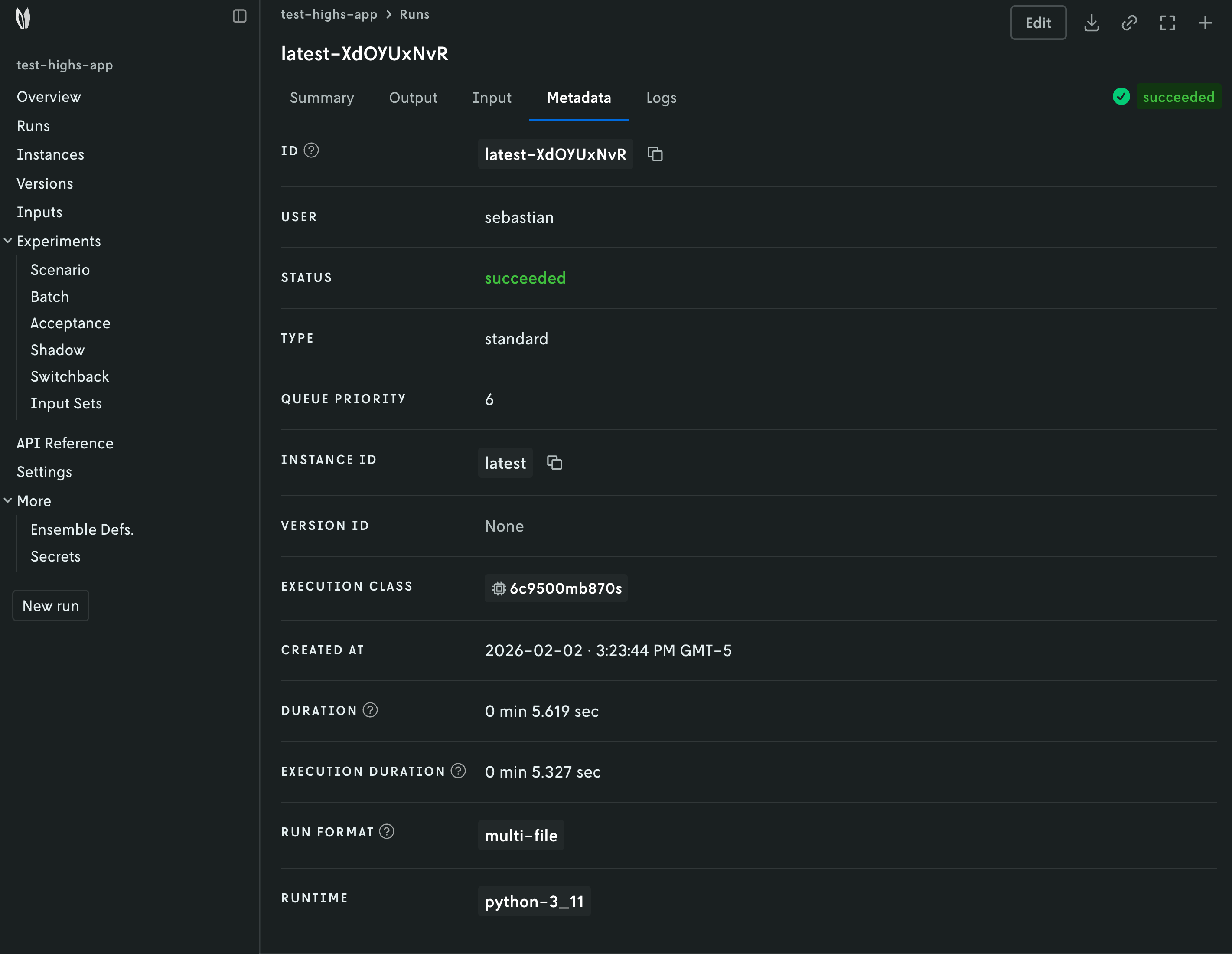
You can go to the apps section in the Nextmv Console where you will see your application. You can click on it to see more details. In the overview of the app you will see the most recent runs. Click on any of the runs that were tracked.
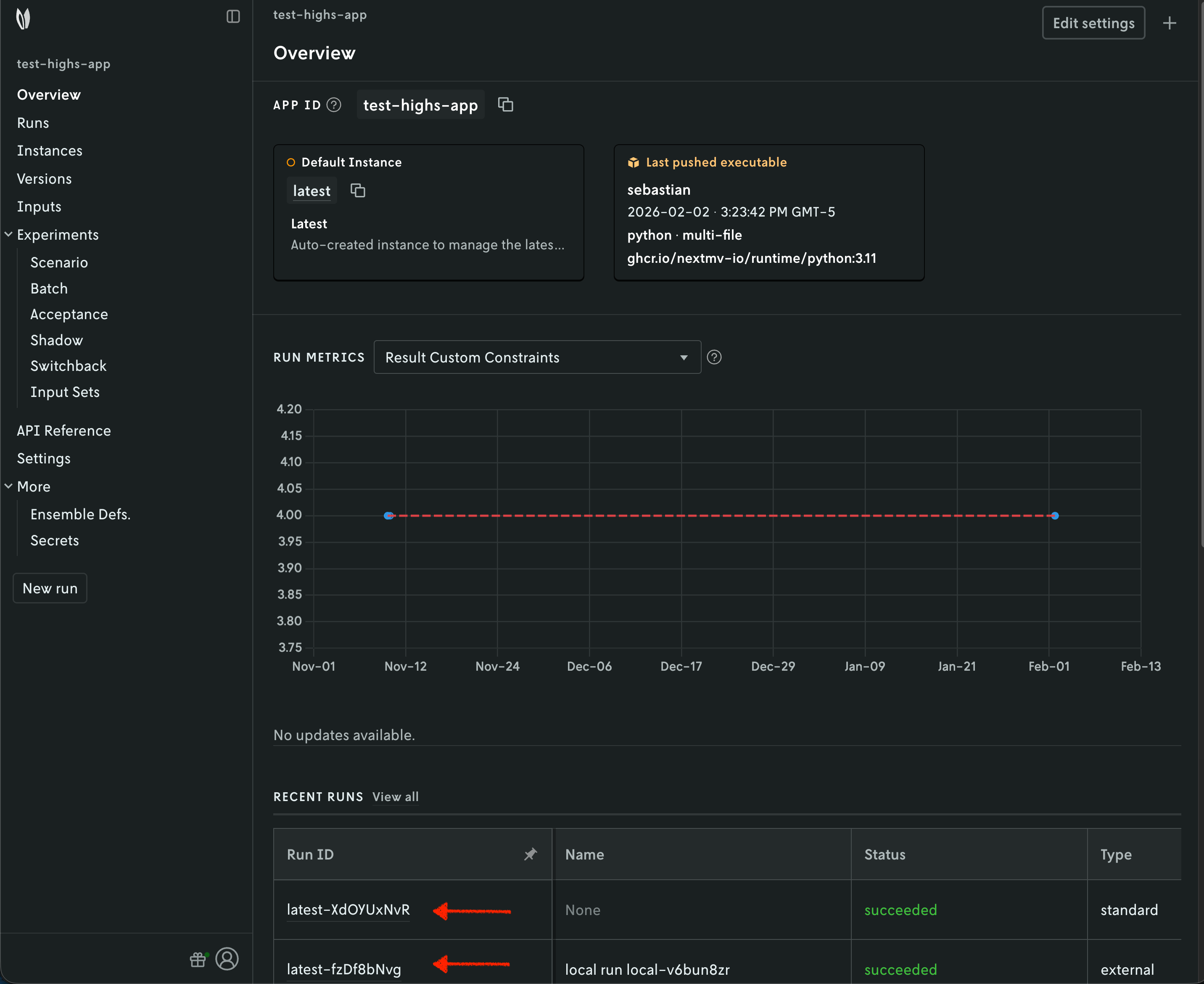
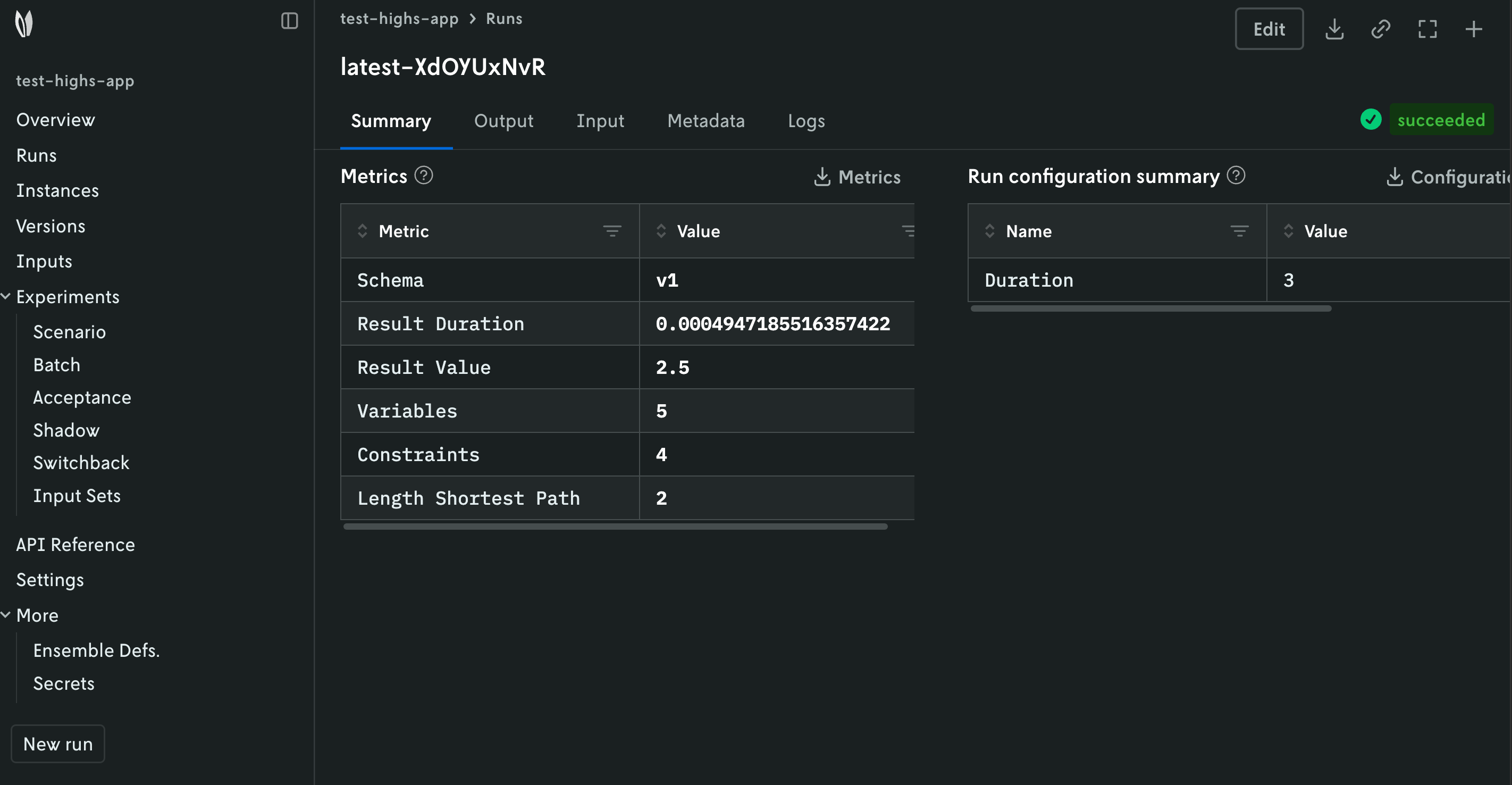
You can use the Nextmv Console to browse the information of the run:
- Summary
- Output
- Input
- Metadata
- Logs
Nextmv is built for collaboration, so you can invite team members to your account and share run URLs.
9. Push your Nextmv application
So far, your application has run locally. You are going to push your app to Nextmv Cloud. Once an application has been pushed, you can run it remotely, perform testing, experimentation, and much more. Pushing is the equivalent of deploying an application, this is, taking the executable code and sending it to Nextmv Cloud.
Create another script, which you can name app5.py, or use another cell in the
Jupyter notebook. Copy and paste the following code into it, making sure you
use the correct dirpath for the Manifest.from_yaml method and app_dir for
the push method:
import os

import nextmv
from nextmv import cloud

# Instantiate the cloud application.
client = cloud.Client(api_key=os.getenv("NEXTMV_API_KEY"))
cloud_app = cloud.Application(client=client, id="test-pyomo-app")

# Push the app.
manifest = nextmv.Manifest.from_yaml(dirpath=".")
cloud_app.push(manifest=manifest, app_dir=".", verbose=True)
import os

import nextmv
from nextmv import cloud

# Instantiate the cloud application.
client = cloud.Client(api_key=os.getenv("NEXTMV_API_KEY"))
cloud_app = cloud.Application(client=client, id="test-highs-app")

# Push the app.
manifest = nextmv.Manifest.from_yaml(dirpath=".")
cloud_app.push(manifest=manifest, app_dir=".", verbose=True)
This script will push the executable code to the application.
After you run the script, or notebook cell, you should see an output similar to this one, where it shows the app being bundled and pushed to Nextmv Cloud.
💽 Starting build for Nextmv application.
🐍 Bundling Python dependencies.
📋 Copied files listed in "app.yaml" manifest.
📦 Packaged application (3296 files, 29.10 MiB).
🌟 Pushing to application: "test-highs-app".
💥️ Successfully pushed to application: "test-highs-app".
{
  "app_id": "test-highs-app",
  "endpoint": "https://api.cloud.nextmv.io",
  "instance_url": "v1/applications/test-highs-app/runs?instance_id=latest"
}
Refreshing the overview of the application in the Nextmv Console should show the following:
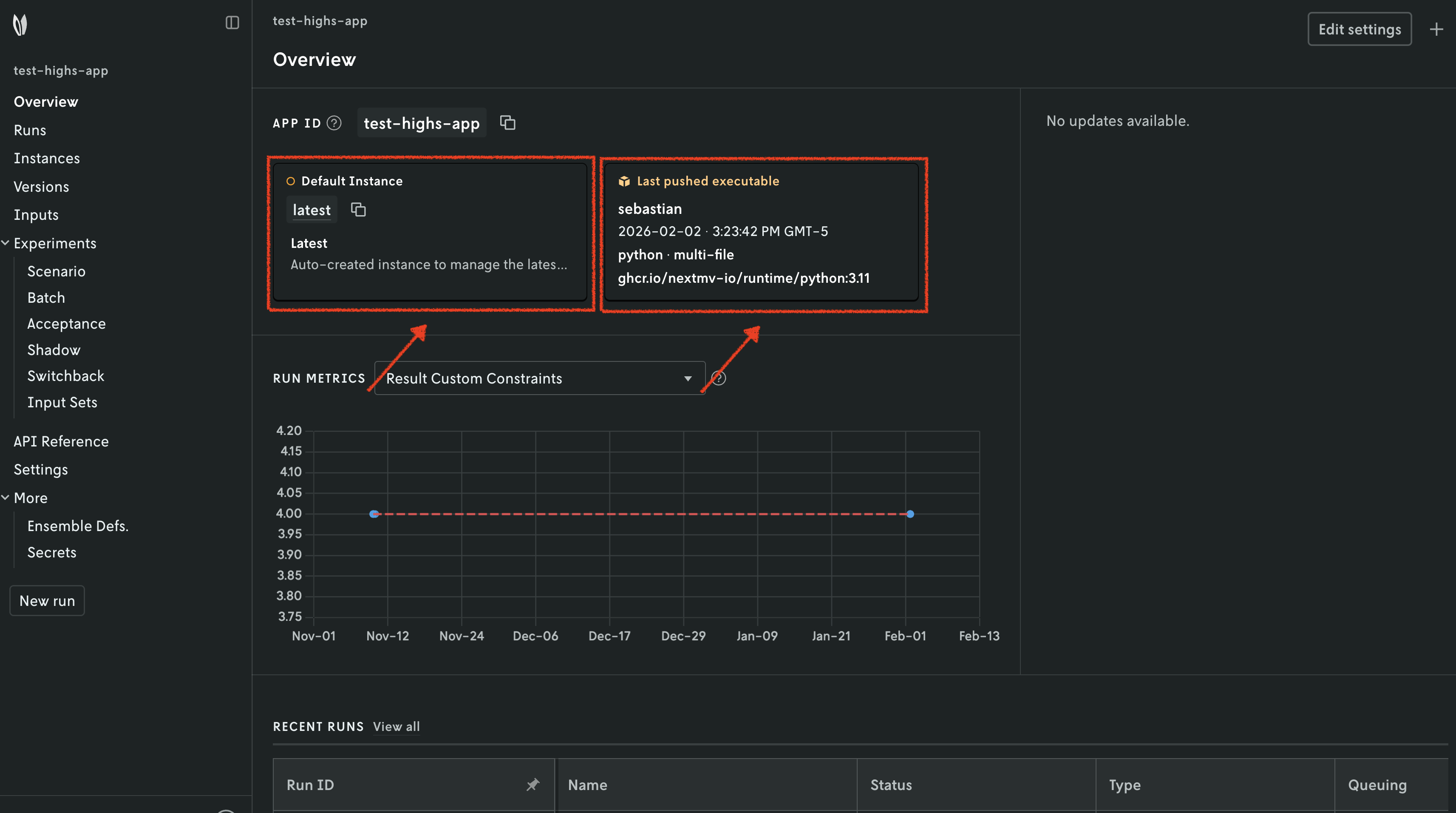
- There is now a pushed executable.
- There is an auto-created
latestinstance, assigned to the executable.
An instance is like the endpoint of the application.
10. Run the Nextmv application remotely
To run the Nextmv application remotely, you have several options. For this
tutorial, we will be using the Nextmv Console and the cloud package of the
Python SDK.
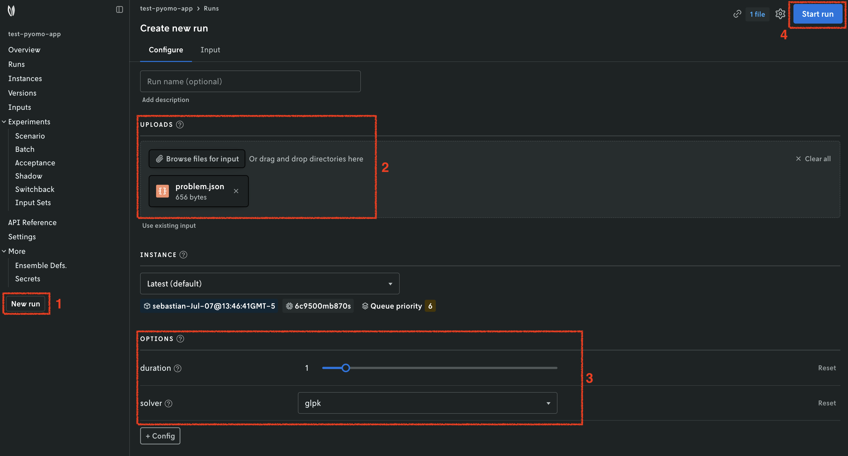
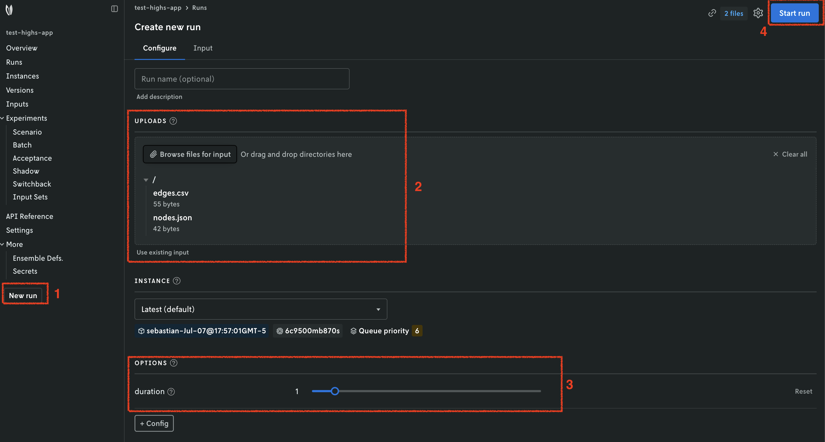
In the Nextmv Console, in the app overview page:
- Press the
New runbutton. - Drop the data files that you want to use. You will get a preview of the
data.
- For Pyomo, use the
problem.jsonfile. - For HiGHS, use both the
nodes.jsonandedges.csvfiles.
- For Pyomo, use the
- Configure your run according to the options that are set in the
app.yamlmanifest.- For Pyomo, you can configure the
durationandsolver. - For HiGHS, you can configure the
duration.
- For Pyomo, you can configure the
- Start the run.
Navigate around to visualize the results of the run. This should look, and feel, like the external (local) run you tracked in a previous step. In this case, the run was executed on Nextmv Cloud.
Alternatively, you can run your Nextmv application using the Python SDK. Create
another script, which you can name app6.py, or use another cell in the
Jupyter notebook. Copy and paste the following code into it:
import os

import nextmv
from nextmv import cloud

# Instantiate the cloud application.
client = cloud.Client(api_key=os.getenv("NEXTMV_API_KEY"))
cloud_app = cloud.Application(client=client, id="test-pyomo-app")

# Run the app.
input = nextmv.load(path=os.path.join("inputs", "problem.json"))
run_result = cloud_app.new_run_with_result(
    input=input.data,  # Data is loaded from memory.
    run_options={
        "duration": "3",
        "solver": "scip",
    },
)
nextmv.write(run_result)
import os

import nextmv
from nextmv import cloud

# Instantiate the cloud application.
client = cloud.Client(api_key=os.getenv("NEXTMV_API_KEY"))
cloud_app = cloud.Application(client=client, id="test-highs-app")

# Run the app.
run_result = cloud_app.new_run_with_result(
    input_dir_path="./inputs",  # Data is loaded from a dir.
    run_options={"duration": "3"},
)
nextmv.write(run_result)
This script will start a new run on Nextmv Cloud, wait for it to complete, and print the results. After you run the script, or notebook cell, you should see an output similar to this one:
{
  "description": "",
  "id": "latest-fEh2_xWDR",
  "metadata": {
    "application_id": "test-pyomo",
    "application_instance_id": "latest",
    "application_version_id": "",
    "created_at": "2025-12-02T17:36:27Z",
    "duration": 22020.0,
    "error": "",
    "input_size": 462.0,
    "output_size": 667.0,
    "format": {
      "input": {
        "type": "json"
      },
      "output": {
        "type": "json"
      }
    },
    "status_v2": "succeeded",
    "status": "succeeded",
    "statistics": {
      "schema": "v1",
      "result": {
        "duration": 0.04,
        "value": 153.675,
        "custom": {
          "variables": 6,
          "constraints": 5,
          "num_edges_used": 3
        }
      }
    }
  },
  "name": "",
  "user_email": "sebastian@nextmv.io",
  "console_url": "https://cloud.nextmv.io/app/test-pyomo/run/latest-fEh2_xWDR?view=details",
  "output": {
    "options": {
      "duration": 3.0,
      "solver": "scip",
      "input": "",
      "output": ""
    },
    "solution": {
      "shipments": [
        {
          "from": "seattle",
          "to": "chicago",
          "quantity": 300.0
        },
        {
          "from": "san-diego",
          "to": "new-york",
          "quantity": 325.0
        },
        {
          "from": "san-diego",
          "to": "topeka",
          "quantity": 275.0
        }
      ]
    },
    "statistics": {
      "result": {
        "duration": 0.04,
        "value": 153.675,
        "custom": {
          "variables": 6,
          "constraints": 5,
          "num_edges_used": 3
        }
      },
      "schema": "v1"
    },
    "assets": []
  }
}
{
  "description": "",
  "id": "latest-tpymlxZvR",
  "metadata": {
    "application_id": "test-highs",
    "application_instance_id": "latest",
    "application_version_id": "",
    "created_at": "2025-12-02T17:30:03Z",
    "duration": 21027.0,
    "error": "",
    "input_size": 322.0,
    "output_size": 164.0,
    "format": {
      "input": {
        "type": "multi-file"
      },
      "output": {
        "type": "multi-file"
      }
    },
    "status_v2": "succeeded",
    "status": "succeeded",
    "statistics": {
      "schema": "v1",
      "result": {
        "duration": 0.00038242340087890625,
        "value": 2.5,
        "custom": {
          "variables": 5,
          "constraints": 4,
          "length_shortest_path": 2
        }
      }
    }
  },
  "name": "",
  "user_email": "sebastian@nextmv.io",
  "console_url": "https://cloud.nextmv.io/app/test-highs/run/latest-tpymlxZvR?view=details",
  "output": {
    "url": "..."
  }
}
11. Perform a scenario test
We are going to take full advantage of the Nextmv Platform by creating a scenario test. Scenario tests are generally used as an exploratory test to understand the impacts to business metrics (or KPIs) on situations such as:
- Updating a model with a new feature, such as an additional constraint.
- Comparing how the same model performs in different conditions, such as low demand vs. high demand.
- Doing a sensitivity analysis to understand how the model behaves when changing a parameter.
Start by creating an input set. As the name suggests, it is a set of inputs,
and it serves as a base so that we can perform runs varying one or more
configurations (options). To create an input set, you have several options. For
this tutorial, we will be using the Nextmv Console and the cloud package of
the Python SDK. You may follow these steps for both examples.
- Navigate to the
Input setssection. - Set a name for your input set.
- Use the
Instance + date rangecreation type given that we already have a few runs on thelatestinstance. - Create the input set.
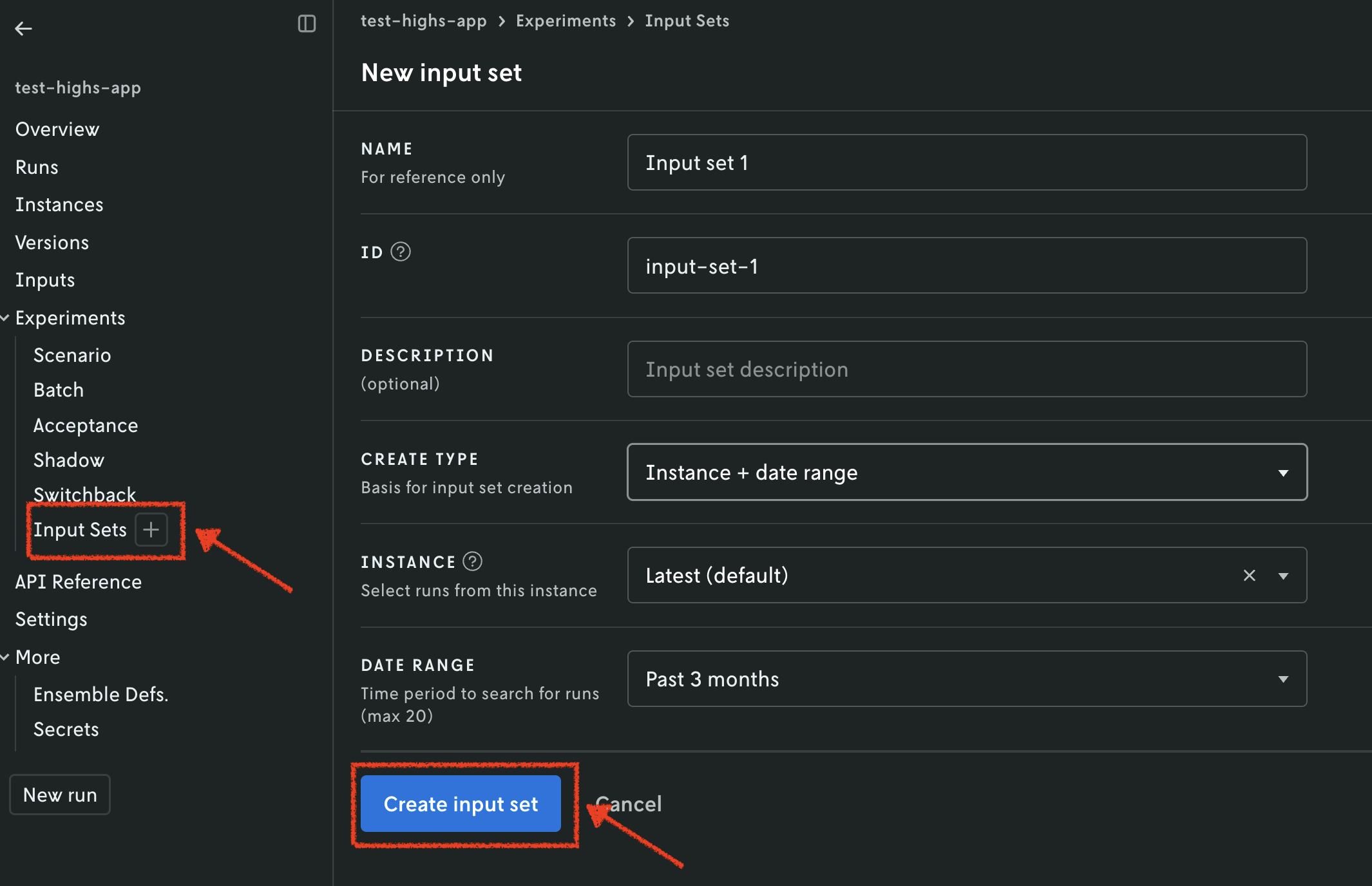
Another option for creating the input set is using the Python SDK. Create
another script, which you can name app7.py, or use another cell in the
Jupyter notebook. Copy and paste the following code into it:
import os
from datetime import datetime, timedelta, timezone

import nextmv
from nextmv import cloud

# Instantiate the cloud application.
client = cloud.Client(api_key=os.getenv("NEXTMV_API_KEY"))
cloud_app = cloud.Application(client=client, id="test-pyomo-app")

# Create the input set.
input_set = cloud_app.new_input_set(
    instance_id="latest",
    start_time=datetime.now(timezone.utc) - timedelta(days=1),
    end_time=datetime.now(timezone.utc),
)
nextmv.write(input_set)
import os
from datetime import datetime, timedelta, timezone

import nextmv
from nextmv import cloud

# Instantiate the cloud application.
client = cloud.Client(api_key=os.getenv("NEXTMV_API_KEY"))
cloud_app = cloud.Application(client=client, id="test-highs-app")

# Create the input set.
input_set = cloud_app.new_input_set(
    instance_id="latest",
    start_time=datetime.now(timezone.utc) - timedelta(days=1),
    end_time=datetime.now(timezone.utc),
)
nextmv.write(input_set)
This script will create a new input set. After you run the script, or notebook cell, you should see an output similar to this one:
Once your input set has been created, we are going to create a scenario test.
Similarly to runs, and input sets, you have several options to achieve this. We
will continue to use the Nextmv Console and the cloud
package of the Python SDK in this tutorial. You may follow
these steps for both examples.
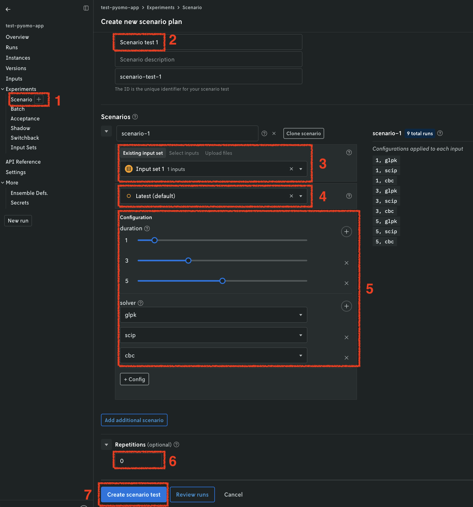
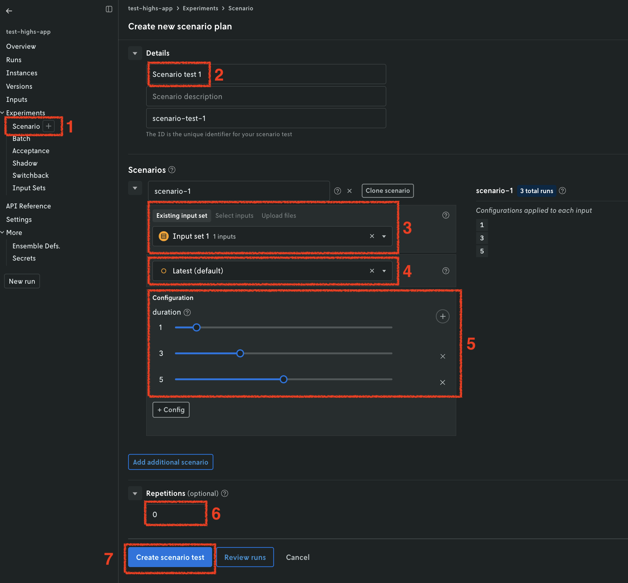
- Navigate to the
Scenariosection. - Set a name for your scenario test.
- Select the input set you just created in the previous step.
- Select the
latestinstance. - Create configuration combinations, which will be factored in to create the
scenarios.
- For Pyomo, we are setting
durationto be 1, 3, and 5 seconds; and forsolverwe are comparing the three supported solvers:glpk,scipandcbc. - For HiGHS, we are setting
durationto be 1, 3, and 5 seconds.
- For Pyomo, we are setting
- Optionally, you may configure repetitions. These are useful when the results are not deterministic.
- Create the scenario test. Review and confirm the number of scenarios that will be created.
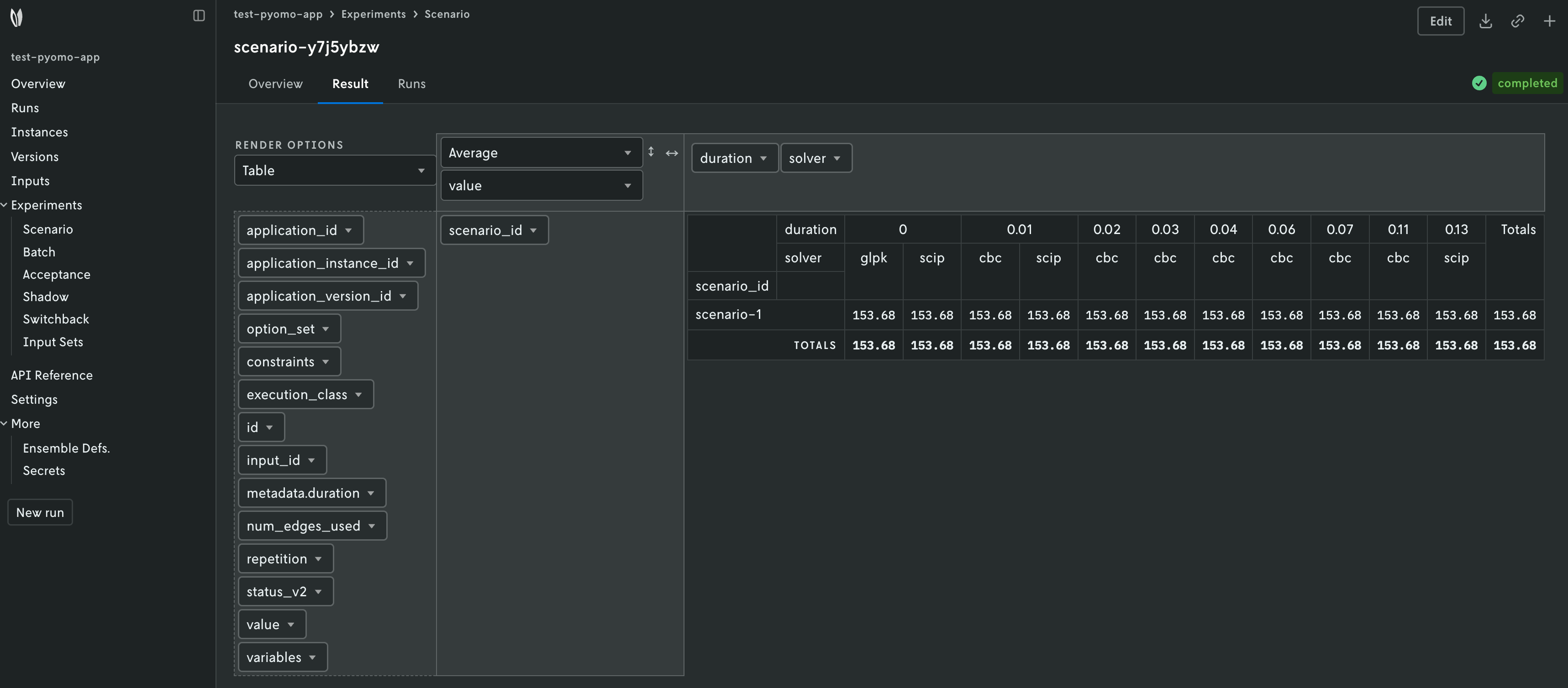
Once all the runs in the scenario test are completed, you can visualize the result of the test. A pivot table is provided to create useful comparisons of your metrics across the scenario test runs.
As an alternative, you may create the scenario test using the Python SDK.
Create another script, which you can name app8.py, or use another cell in the
Jupyter notebook. Copy and paste the following code into it:
import os

from nextmv import cloud

# Instantiate the cloud application.
client = cloud.Client(api_key=os.getenv("NEXTMV_API_KEY"))
cloud_app = cloud.Application(client=client, id="test-pyomo-app")

# Create the scenario test.
scenario_test_id = cloud_app.new_scenario_test(
    scenarios=[
        cloud.Scenario(
            scenario_input=cloud.ScenarioInput(
                scenario_input_type=cloud.ScenarioInputType.INPUT_SET,
                scenario_input_data="<INPUT_SET_ID_CREATED_PREVIOUSLY>",
            ),
            instance_id="latest",
            configuration=[
                cloud.ScenarioConfiguration(
                    name="duration",
                    values=["1", "3", "5"],
                ),
                cloud.ScenarioConfiguration(
                    name="solver",
                    values=["glpk", "scip", "cbc"],
                ),
            ],
        ),
    ],
)
print(f"Created scenario test with ID: {scenario_test_id}")
import os

from nextmv import cloud

# Instantiate the cloud application.
client = cloud.Client(api_key=os.getenv("NEXTMV_API_KEY"))
cloud_app = cloud.Application(client=client, id="test-highs-app")

# Create the scenario test.
scenario_test_id = cloud_app.new_scenario_test(
    scenarios=[
        cloud.Scenario(
            scenario_input=cloud.ScenarioInput(
                scenario_input_type=cloud.ScenarioInputType.INPUT_SET,
                scenario_input_data="<INPUT_SET_ID_CREATED_PREVIOUSLY>",
            ),
            instance_id="latest",
            configuration=[
                cloud.ScenarioConfiguration(
                    name="duration",
                    values=["1", "3", "5"],
                ),
            ],
        ),
    ],
)
print(f"Created scenario test with ID: {scenario_test_id}")
This script will create a new scenario test. After you run the script, or notebook cell, you should see an output similar to this one:
🎉🎉🎉 Congratulations, you have finished this tutorial!
Full tutorial code
You can find the consolidated code examples used in this tutorial in the
tutorials GitHub repository. The
connect-your-model-python dir contains all the
code that was shown in this tutorial.
For each of the examples, you will find two directories:
original: the original example without any modifications.nextmv-ified: the example converted into a Nextmv application.
Go into each directory for instructions about running the decision model.