Add custom visualizations to runs¶

In this tutorial you will learn how to use the Nextmv CLI and community apps to to add custom visualizations to your Nextmv run output, so you can view interactive charts and maps directly in the Console. Complete this tutorial if you:

• Don’t have a pre-existing decision model and you want to explore visualizations in the Nextmv Platform.
• Are fluent using Python 🐍.
• Are familiar using uv for managing Python.

Community apps are Nextmv applications that showcase how to solve different decision problems with various languages and solvers. They are a great way to explore new decision models and the Nextmv Platform. You can think of community apps as examples that serve as strong references when building and customizing your own decision models.

At a high level, this tutorial will go through the following steps:

1. Clone a community app locally.
2. Add visualizations to it.
3. Run it and visualize the app locally.
4. Push the model to Nextmv Cloud.
5. Run the model and visualize it remotely.

You may follow along with the full tutorial code. Let’s dive right in 🤿.

1. Create an account¶

The full suite of benefits starts with a Nextmv Cloud account.

1. Visit the Nextmv Console to sign up for an account at https://cloud.nextmv.io.
2. Fill out the form. A member of the Nextmv team will reach out to you to complete the sign-up process.
3. Log in to your account. The Nextmv Console is ready to use!

Once you have logged in to your account, you need to fetch your API key. You can do so from your settings.

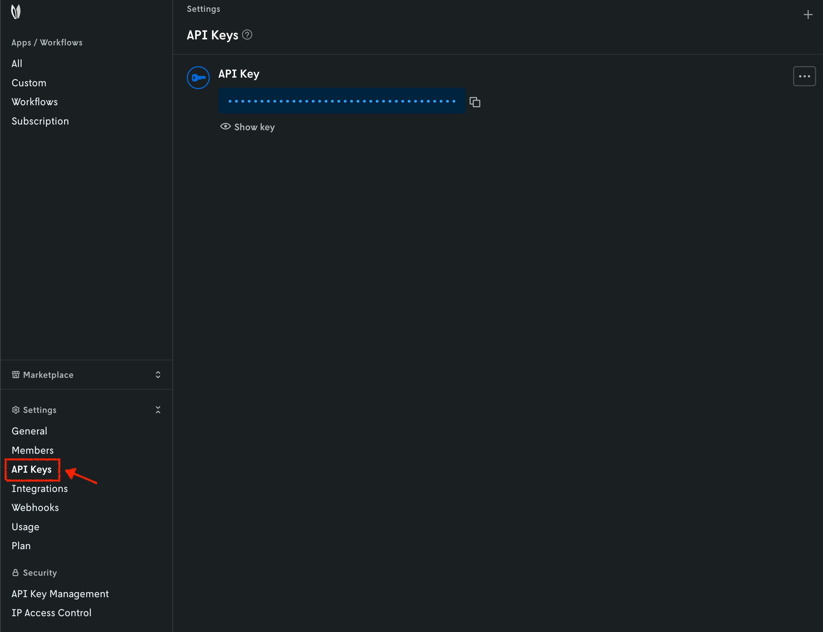
When you have your API key, it is convenient to save it as an environment variable so that you can use it for the rest of this tutorial.

export NEXTMV_API_KEY="<YOUR-API-KEY>"

$env:NEXTMV_API_KEY = "<YOUR-API-KEY>"

2. Install the Nextmv CLI¶

Please see the Nextmv CLI installation guide.

3. Clone a community app¶

To work with community apps you have two options:

1. Clone the GitHub repository locally.
2. Use the Nextmv CLI to clone a specific community app.

This tutorial will use the second option.

For this tutorial, we will be using the python-highs-knapsack community app, which solves a knapsack problem using the HiGHS solver and Python. To clone this community app, run the following command:

nextmv community clone -a python-highs-knapsack -d original
nextmv community clone -a python-highs-knapsack -d visualization

✅ Successfully cloned the python-highs-knapsack community app, using version latest in path: original.
✅ Registered the cloned community app python-highs-knapsack as a local app with ID local-app-xxxx.
✅ Successfully cloned the python-highs-knapsack community app, using version latest in path: visualization.
✅ Registered the cloned community app python-highs-knapsack as a local app with ID local-app-xxxx.

This command is saved as app1.sh in the full tutorial code.

You'll notice that we are cloning the app twice, once to have a reference for the original app, and once so we can modify it and add visualizations to it, which we will call visualization.

With the apps cloned, you should see a structure similar to the following:

.
├── app.yaml
├── input.json
├── LICENSE
├── main.ipynb
├── main.py
├── pyproject.toml
├── README.md
├── requirements.txt
└── uv.lock

4. Run the community app locally¶

You can use the nextmv local run create command to start a local run. At the root of the original app (where the original/app.yaml manifest is located), run the following command:

# Run this command from the root of both apps, this is, where the
# original/app.yaml and visualization/app.yaml files are located.
nextmv local run create -i input.json --wait

✅ Run local-680yln1r created.
⏳ Getting run results...
{
  "description": "Local run created at 2026-07-10T16:25:10.897034Z",
  "id": "local-680yln1r",
  "metadata": {
    "application_id": "local-app-b5amqr3a",
    "application_instance_id": "",
    "application_version_id": "",
    "created_at": "2026-07-10T16:25:10.897034Z",
    "duration": 1046.2,
    "error": "",
    "execution_class": "local",
    "execution_duration": 1046.2,
    "experiment_id": "",
    "experiment_type": "",
    "format": {
      "input": {
        "type": "json"
      },
      "output": {
        "type": "json"
      }
    },
    "initiated_at": "2026-07-10T16:25:10.897034Z",
    "input_size": 820.0,
    "metrics": {
      "duration": 0.0028638839721679688,
      "value": 444,
      "status": "HighsStatus.kOk",
      "variables": 11,
      "constraints": 1,
      "solver_version": "1.9.0"
    },
    "options": {
      "active_options": {},
      "options_summary": [],
      "request_options": {}
    },
    "output_size": 0.0,
    "queuing_disabled": true,
    "queuing_priority": 0,
    "run_type": {
      "type": "standard",
      "definition_id": "",
      "reference_id": ""
    },
    "runtime": "local",
    "secrets_collection_id": "",
    "status_v2": "succeeded",
    "tracking": {
      "cloned_run_id": "",
      "input_id": ""
    }
  },
  "name": "local run local-680yln1r",
  "user_email": "",
  "console_url": "",
  "output": {
    "options": {
      "duration": 30
    },
    "solution": {
      "items": [
        {
          "id": "cat",
          "value": 100,
          "weight": 20
        },
        {
          "id": "water",
          "value": 40,
          "weight": 2
        },
        {
          "id": "phone",
          "value": 6,
          "weight": 1
        },
        {
          "id": "book",
          "value": 63,
          "weight": 10
        },
        {
          "id": "rx",
          "value": 81,
          "weight": 1
        },
        {
          "id": "coat",
          "value": 44,
          "weight": 9
        },
        {
          "id": "keys",
          "value": 92,
          "weight": 1
        },
        {
          "id": "nuts",
          "value": 18,
          "weight": 4
        }
      ]
    },
    "assets": [],
    "metrics": {
      "duration": 0.0028638839721679688,
      "value": 444,
      "status": "HighsStatus.kOk",
      "variables": 11,
      "constraints": 1,
      "solver_version": "1.9.0"
    }
  }
}

This command is saved as app2.sh in the full tutorial code.

You can make as many runs as you want, and the CLI will keep a record of everything that happens with your local app.

5. Add visualizations to your application¶

There are currently three supported custom visual types:

• GeoJSON: Create your own interactive maps using the common standard for geospatial data exchange.
• Plotly: Create your own plots and more with the powerful JavaScript library.
• Chart.js: Create charts, plots and more with the performant JavaScript library.

Visualizations are automatically picked up by Nextmv if they are included in the output according to the convention of each supported content format:

• json: there is an assets key in the output that contains a list of assets.
• multi-file: there is an assets path described in the app.yaml manifest and the application writes a .json file to that path.

In both cases, the assets must follow the expected schema.

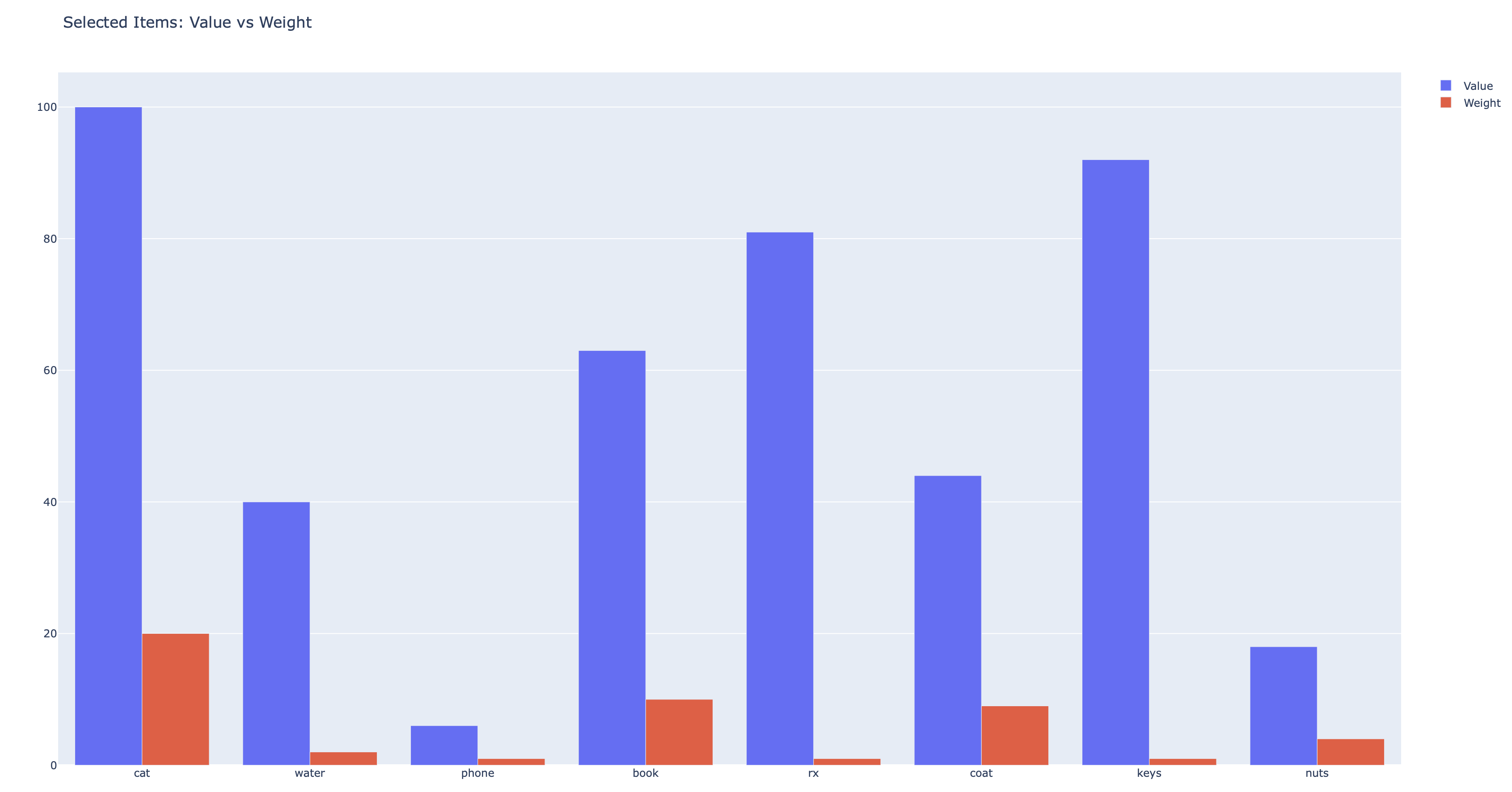
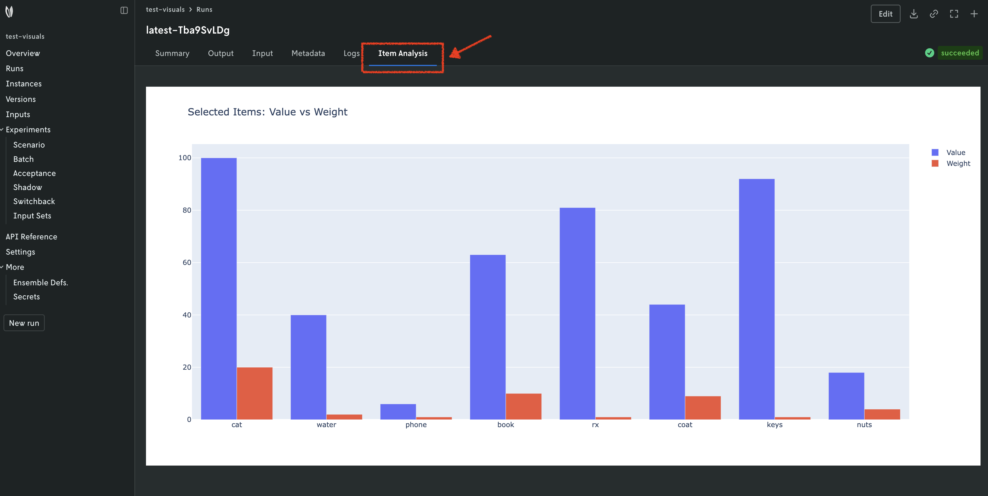
For this tutorial, we will be using the Plotly library to create a simple bar chart that depicts the selected items by value and weight.

Replace the visualization/main.py file with the following code.

import json
import time
from importlib.metadata import version
from typing import Any

import highspy
import nextmv
import plotly.graph_objects as go


def main() -> None:
    """Entry point for the program."""

    loaded_input = nextmv.load()
    options = loaded_input.options

    nextmv.log("Solving knapsack problem:")
    nextmv.log(f"  - items: {len(loaded_input.data.get('items', []))}")
    nextmv.log(f"  - capacity: {loaded_input.data.get('weight_capacity', 0)}")

    solution, metrics, assets = solve(loaded_input)
    nextmv.write(solution=solution, metrics=metrics, assets=assets, options=options)


def solve(
    loaded_input: nextmv.Input,
) -> tuple[dict[str, Any], dict[str, Any], list[nextmv.Asset]]:
    """Solves the given problem and returns the solution, metrics, and assets."""

    start_time = time.time()

    # Creates the solver.
    solver = highspy.Highs()
    solver.silent()  # Solver output ignores stdout redirect, silence it.
    solver.setOptionValue("time_limit", loaded_input.options.duration)

    # Initializes the linear sums.
    weights = 0.0
    values = 0.0

    # Creates the decision variables and adds them to the linear sums.
    items = []
    for item in loaded_input.data["items"]:
        item_variable = solver.addVariable(0.0, 1.0, item["value"])
        items.append({"item": item, "variable": item_variable})
        weights += item_variable * item["weight"]
        values += item_variable * item["value"]

    # This constraint ensures the weight capacity of the knapsack will not be
    # exceeded.
    solver.addConstr(weights <= loaded_input.data["weight_capacity"])

    # Sets the objective function: maximize the value of the chosen items.
    status = solver.maximize(values)

    # Determines which items were chosen.
    chosen_items = [
        item["item"] for item in items if solver.val(item["variable"]) > 0.9
    ]

    solution = {"items": chosen_items}

    metrics = {
        "duration": time.time() - start_time,
        "value": sum(item["value"] for item in chosen_items),
        "status": str(status),
        "variables": solver.numVariables,
        "constraints": solver.numConstrs,
        "solver_version": version("highspy"),
    }

    # After solving, create visualization.
    fig = go.Figure()
    fig.add_trace(
        go.Bar(
            x=[item["id"] for item in chosen_items],
            y=[item["value"] for item in chosen_items],
            name="Value",
        )
    )
    fig.add_trace(
        go.Bar(
            x=[item["id"] for item in chosen_items],
            y=[item["weight"] for item in chosen_items],
            name="Weight",
        )
    )
    fig.update_layout(
        title="Selected Items: Value vs Weight",
        barmode="group",
    )

    assets = [
        nextmv.Asset(
            name="item-chart",
            content=[json.loads(fig.to_json())],
            visual=nextmv.Visual(
                visual_schema=nextmv.VisualSchema.PLOTLY,
                label="Item Analysis",
            ),
        )
    ]

    return solution, metrics, assets


if __name__ == "__main__":
    main()

Now you can start a local run from the root of the visualization app (where the visualization/app.yaml manifest is located):

# Run this command from the root of both apps, this is, where the
# original/app.yaml and visualization/app.yaml files are located.
nextmv local run create -i input.json --wait

✅ Run local-pz4vkvoy created.
⏳ Getting run results...
💡 Removed assets from output for cleaner display, use --output to save the full output.
{
  "description": "Local run created at 2026-07-10T16:47:46.123832Z",
  "id": "local-pz4vkvoy",
  "metadata": {
    "application_id": "local-app-6rnociuv",
    "application_instance_id": "",
    "application_version_id": "",
    "created_at": "2026-07-10T16:47:46.123832Z",
    "duration": 1283.5,
    "error": "",
    "execution_class": ""
  ... Output truncated for brevity ...
}

You'll notice that there is a message indicating that the assets were removed from the output for a clear display. You can visualize the assets of a run by using the nextmv local run visuals command to visualize the assets of a run.

# Run this command from the root of the visualization app, this is, where the visualization/app.yaml file is located.
nextmv local run visuals -r "<RUN_ID_PRINTED_PREVIOUSLY>"

⏳ Getting run visuals...
✅ Run visuals opened in web browser, here are the local URLs of the visual files:
[
  "file:///user/custom-visualizations-cli/visualization/.nextmv/runs/local-pz4vkvoy/visuals/Item Analysis_0.html"
]

This will open a browser window for each asset produced by the run. You should see a simple plot like the following:

This command is saved as app3.sh in the full tutorial code.

Support for custom visuals extends all the way to Nextmv Console, so you can visualize your runs remotely as well.

6. Create your Nextmv Cloud application¶

Run the following command:

nextmv cloud app create -a test-visuals --exist-ok

⏳ Creating or getting application...
{
  "id": "test-visuals",
  "name": "test-visuals",
  "description": "",
  "type": "custom",
  "default_instance": "latest",
  "default_experiment_instance": "",
  "subscription_id": "",
  "locked": false,
  "created_at": "2026-07-09T18:40:36.158310Z",
  "updated_at": "2026-07-09T18:42:58.375241Z"
}

This will create a new application in Nextmv Cloud. Note that the name and app ID can be different, but for simplicity this tutorial uses the same name and app ID. This command is saved as app4.sh in the full tutorial code. You can also create applications directly from Nextmv Console.

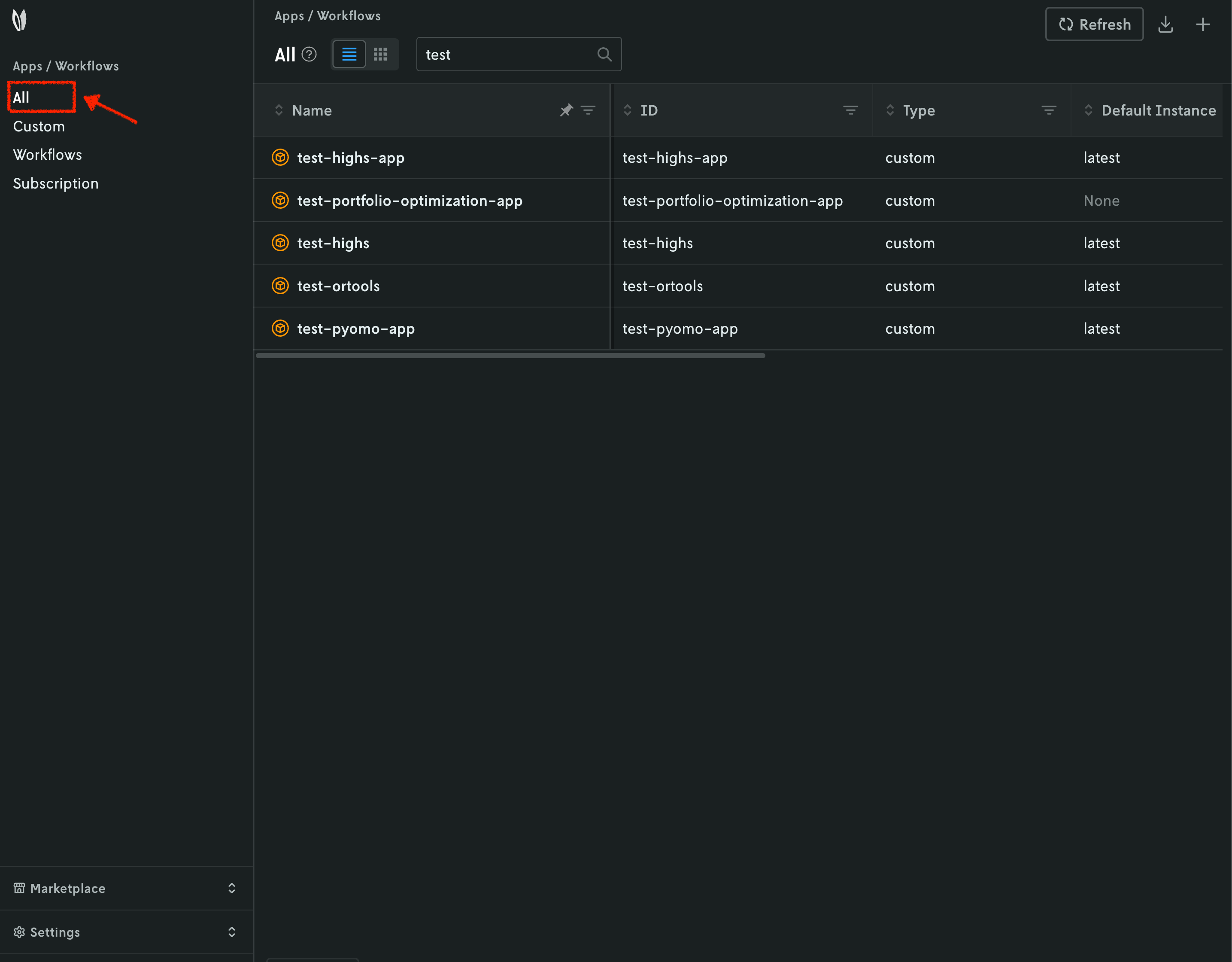
You can go to the Apps section in the Nextmv Console where you will see your applications.

7. Push your Nextmv application¶

So far, your application has run locally. You are going to push your app to Nextmv Cloud. Once an application has been pushed, you can run it remotely, perform testing, experimentation, and much more. Pushing is the equivalent of deploying an application, this is, taking the executable code and sending it to Nextmv Cloud.

At the root of the visualization app (where the visualization/app.yaml manifest is located), deploy your app (push it) to Nextmv Cloud:

# Run this command from the root of the visualization app, this is, where the visualization/app.yaml file is located.
nextmv cloud app push -a test-visuals

💽 Starting build for Nextmv application.
🐍 Bundling Python dependencies.
📋 Copied files listed in "app.yaml" manifest.
📦 Packaged application (25.49 MiB, 2120 files).
🌟 Pushing to application: "test-visuals".
💥️ Successfully pushed to application: "test-visuals".
{
  "app_id": "test-visuals",
  "endpoint": "api.cloud.nextmv.io",
  "instance_url": "https://api.cloud.nextmv.io/v1/applications/test-visuals/runs?instance_id=latest"
}

This command is saved as app5.sh in the full tutorial code.

You can go to the Apps section in the Nextmv Console where you will see your application. You can click on it to see more details. Once you are in the overview of the application in the Nextmv Console, it should show the following:

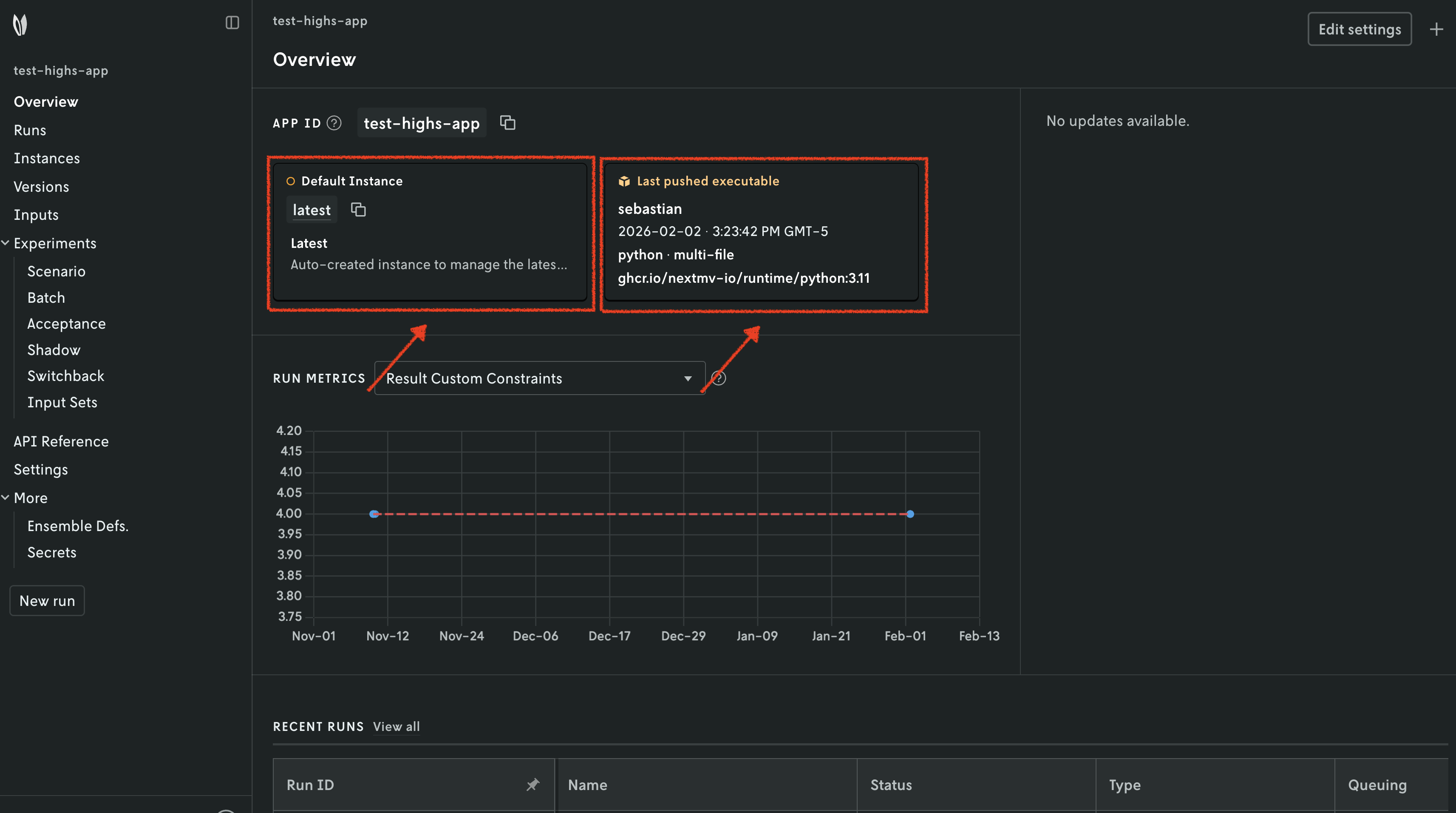
• There is now a pushed executable.
• There is an auto-created latest instance, assigned to the executable.

An instance is like the endpoint of the application.

8. Run the Nextmv application remotely¶

To run the Nextmv application remotely, you have several options. For this tutorial, we will be using the Nextmv Console and CLI.

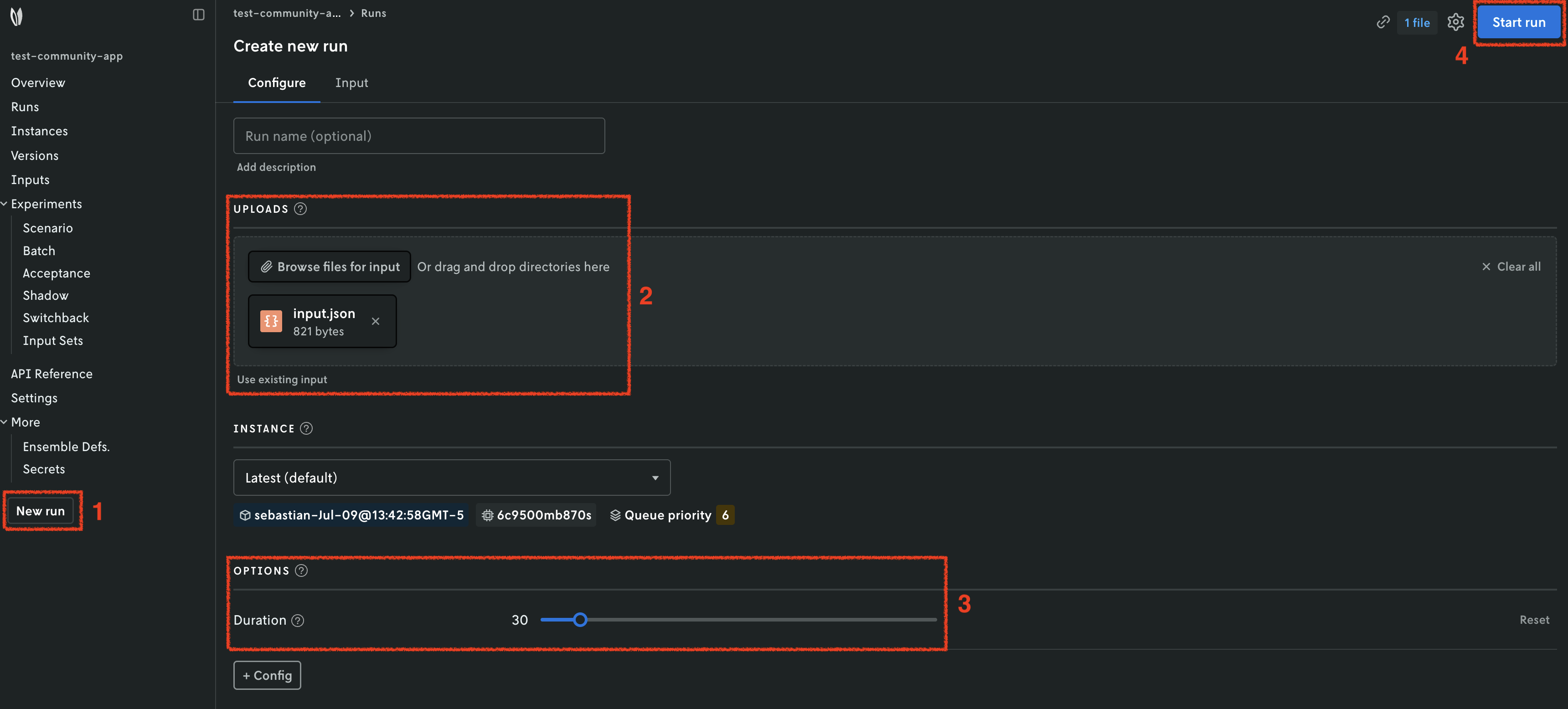
In the Nextmv Console, in the app overview page:

1. Press the New run button.
2. Drop the data files that you want to use. You will get a preview of the data. You can drop the input.json file that comes with the community app.
3. Optionally, configure your run according to the options that can be passed. In this case, you can configure the duration.
4. Start the run.

A tab called Item Analysis will be available, which is the custom visualization that we added to the application. You can click on it to see the interactive chart.

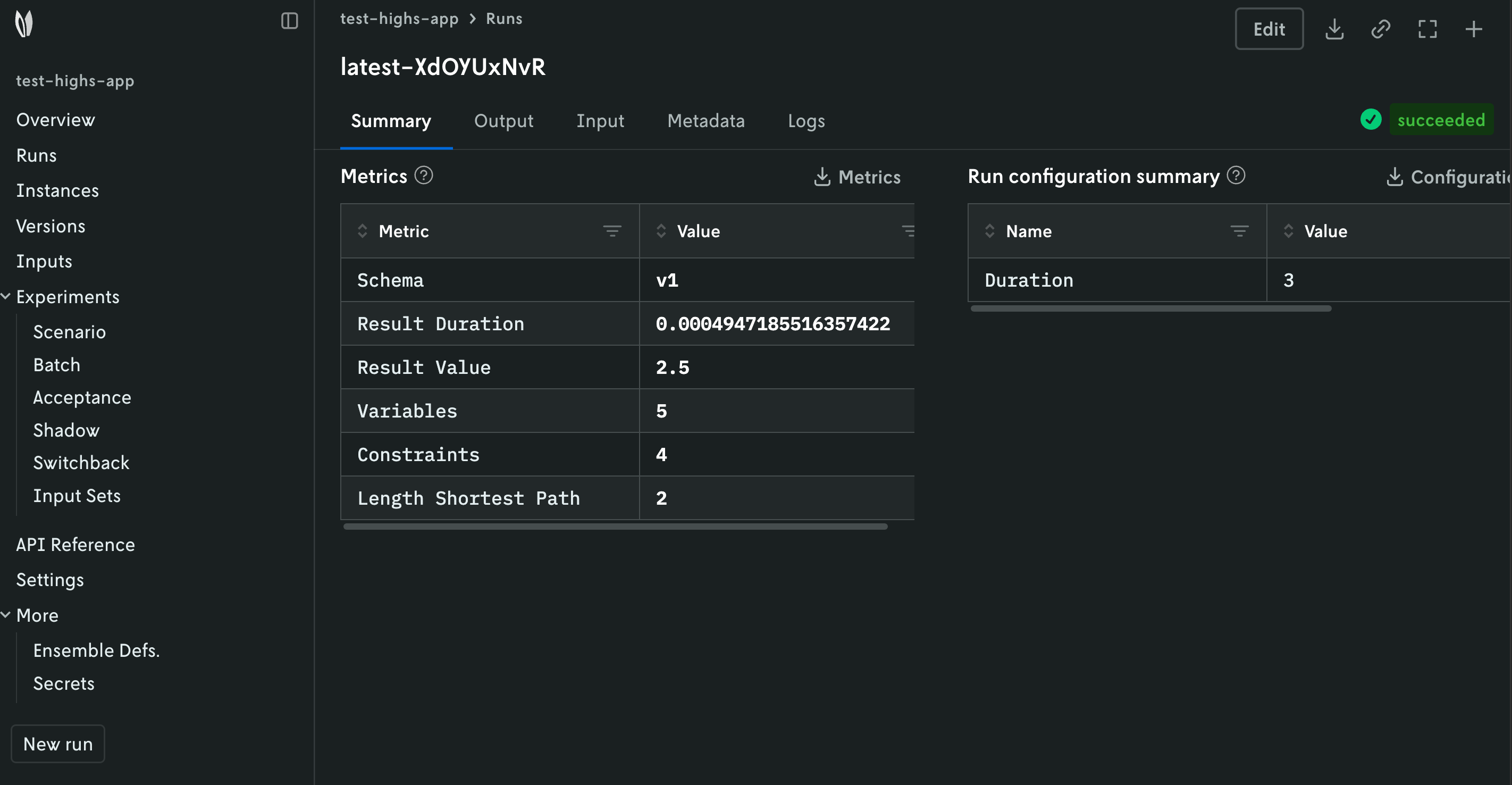
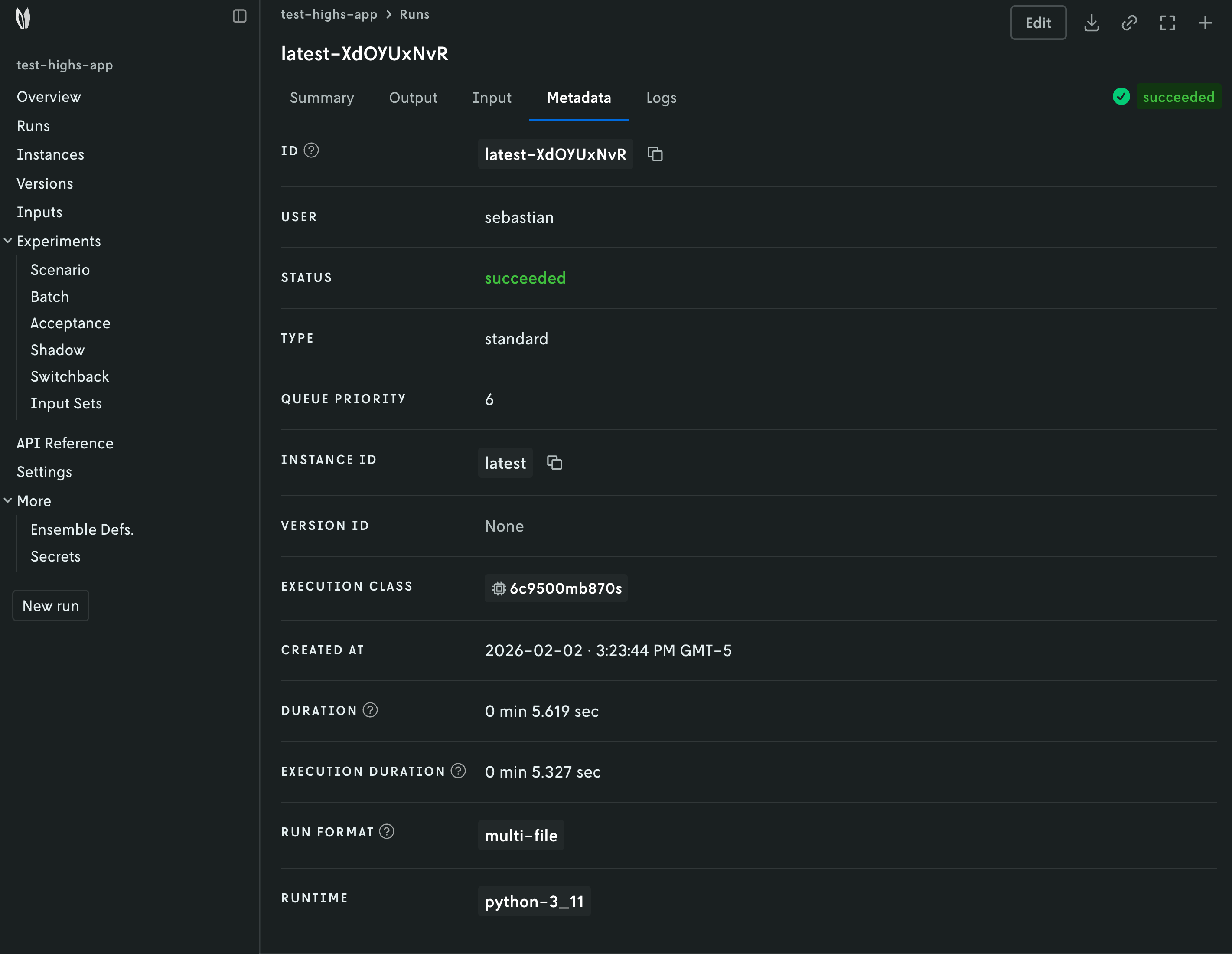
You can also use the Nextmv Console to browse the information of the run:

• Summary
• Output
• Input
• Metadata
• Logs

Nextmv is built for collaboration, so you can invite team members to your account and share run URLs.

Alternatively, you can run your Nextmv application using the Nextmv CLI. Here is an example command you can run from the root of the app.

# Run this command from the root of the visualization app, this is, where the visualization/app.yaml file is located.
nextmv cloud run create -a test-visuals -i input.json

{
  "run_id": "latest-jjk3M1Zvg"
}

This command is saved as app6.sh in the full tutorial code.

Full tutorial code¶

You can find the consolidated code examples used in this tutorial in the tutorials GitHub repository. The custom-visualizations-cli dir contains all the code that was shown in this tutorial.

Go into the directory for instructions about running the decision model.