Free local experience with the Nextmv CLI
⌛️ Approximate time to complete: 15 min.
In this tutorial you will learn how to use the Nextmv CLI, in
particular, the nextmv local command tree, to work with Nextmv
applications locally. Complete this tutorial if you:
- Want to explore Nextmv, by starting with a free alternative.
- Are fluent using Python 🐍.
- Are familiar using
uvfor managing Python.
To complete this tutorial, we will use an external example, working under the principle that it is not a Nextmv-created decision model. You can, and should, use your own decision model, or follow along with the example provided:
You may follow along with the full tutorial code. Let’s dive right in 🤿.
1. Install the Nextmv CLI
Please see the Nextmv CLI installation guide.
2. Prepare the executable code
Info
If you are working with your own decision model and already know that it executes, feel free to skip this step.
The decision model is composed of executable code that solves an optimization
problem. Copy the desired example code to a script named main.py.
"""Capacited Vehicles Routing Problem (CVRP)."""

from ortools.constraint_solver import routing_enums_pb2
from ortools.constraint_solver import pywrapcp


def create_data_model():
    """Stores the data for the problem."""
    data = {}
    data["distance_matrix"] = [
        # fmt: off
      [0, 548, 776, 696, 582, 274, 502, 194, 308, 194, 536, 502, 388, 354, 468, 776, 662],
      [548, 0, 684, 308, 194, 502, 730, 354, 696, 742, 1084, 594, 480, 674, 1016, 868, 1210],
      [776, 684, 0, 992, 878, 502, 274, 810, 468, 742, 400, 1278, 1164, 1130, 788, 1552, 754],
      [696, 308, 992, 0, 114, 650, 878, 502, 844, 890, 1232, 514, 628, 822, 1164, 560, 1358],
      [582, 194, 878, 114, 0, 536, 764, 388, 730, 776, 1118, 400, 514, 708, 1050, 674, 1244],
      [274, 502, 502, 650, 536, 0, 228, 308, 194, 240, 582, 776, 662, 628, 514, 1050, 708],
      [502, 730, 274, 878, 764, 228, 0, 536, 194, 468, 354, 1004, 890, 856, 514, 1278, 480],
      [194, 354, 810, 502, 388, 308, 536, 0, 342, 388, 730, 468, 354, 320, 662, 742, 856],
      [308, 696, 468, 844, 730, 194, 194, 342, 0, 274, 388, 810, 696, 662, 320, 1084, 514],
      [194, 742, 742, 890, 776, 240, 468, 388, 274, 0, 342, 536, 422, 388, 274, 810, 468],
      [536, 1084, 400, 1232, 1118, 582, 354, 730, 388, 342, 0, 878, 764, 730, 388, 1152, 354],
      [502, 594, 1278, 514, 400, 776, 1004, 468, 810, 536, 878, 0, 114, 308, 650, 274, 844],
      [388, 480, 1164, 628, 514, 662, 890, 354, 696, 422, 764, 114, 0, 194, 536, 388, 730],
      [354, 674, 1130, 822, 708, 628, 856, 320, 662, 388, 730, 308, 194, 0, 342, 422, 536],
      [468, 1016, 788, 1164, 1050, 514, 514, 662, 320, 274, 388, 650, 536, 342, 0, 764, 194],
      [776, 868, 1552, 560, 674, 1050, 1278, 742, 1084, 810, 1152, 274, 388, 422, 764, 0, 798],
      [662, 1210, 754, 1358, 1244, 708, 480, 856, 514, 468, 354, 844, 730, 536, 194, 798, 0],
        # fmt: on
    ]
    data["demands"] = [0, 1, 1, 2, 4, 2, 4, 8, 8, 1, 2, 1, 2, 4, 4, 8, 8]
    data["vehicle_capacities"] = [15, 15, 15, 15]
    data["num_vehicles"] = 4
    data["depot"] = 0
    return data


def print_solution(data, manager, routing, solution):
    """Prints solution on console."""
    print(f"Objective: {solution.ObjectiveValue()}")
    total_distance = 0
    total_load = 0
    for vehicle_id in range(data["num_vehicles"]):
        if not routing.IsVehicleUsed(solution, vehicle_id):
            continue
        index = routing.Start(vehicle_id)
        plan_output = f"Route for vehicle {vehicle_id}:\n"
        route_distance = 0
        route_load = 0
        while not routing.IsEnd(index):
            node_index = manager.IndexToNode(index)
            route_load += data["demands"][node_index]
            plan_output += f" {node_index} Load({route_load}) -> "
            previous_index = index
            index = solution.Value(routing.NextVar(index))
            route_distance += routing.GetArcCostForVehicle(
                previous_index, index, vehicle_id
            )
        plan_output += f" {manager.IndexToNode(index)} Load({route_load})\n"
        plan_output += f"Distance of the route: {route_distance}m\n"
        plan_output += f"Load of the route: {route_load}\n"
        print(plan_output)
        total_distance += route_distance
        total_load += route_load
    print(f"Total distance of all routes: {total_distance}m")
    print(f"Total load of all routes: {total_load}")


def main():
    """Solve the CVRP problem."""
    # Instantiate the data problem.
    data = create_data_model()

    # Create the routing index manager.
    manager = pywrapcp.RoutingIndexManager(
        len(data["distance_matrix"]), data["num_vehicles"], data["depot"]
    )

    # Create Routing Model.
    routing = pywrapcp.RoutingModel(manager)

    # Create and register a transit callback.
    def distance_callback(from_index, to_index):
        """Returns the distance between the two nodes."""
        # Convert from routing variable Index to distance matrix NodeIndex.
        from_node = manager.IndexToNode(from_index)
        to_node = manager.IndexToNode(to_index)
        return data["distance_matrix"][from_node][to_node]

    transit_callback_index = routing.RegisterTransitCallback(distance_callback)

    # Define cost of each arc.
    routing.SetArcCostEvaluatorOfAllVehicles(transit_callback_index)

    # Add Capacity constraint.
    def demand_callback(from_index):
        """Returns the demand of the node."""
        # Convert from routing variable Index to demands NodeIndex.
        from_node = manager.IndexToNode(from_index)
        return data["demands"][from_node]

    demand_callback_index = routing.RegisterUnaryTransitCallback(demand_callback)
    routing.AddDimensionWithVehicleCapacity(
        demand_callback_index,
        0,  # null capacity slack
        data["vehicle_capacities"],  # vehicle maximum capacities
        True,  # start cumul to zero
        "Capacity",
    )

    # Setting first solution heuristic.
    search_parameters = pywrapcp.DefaultRoutingSearchParameters()
    search_parameters.first_solution_strategy = (
        routing_enums_pb2.FirstSolutionStrategy.PATH_CHEAPEST_ARC
    )
    search_parameters.local_search_metaheuristic = (
        routing_enums_pb2.LocalSearchMetaheuristic.GUIDED_LOCAL_SEARCH
    )
    search_parameters.time_limit.FromSeconds(1)

    # Solve the problem.
    solution = routing.SolveWithParameters(search_parameters)

    # Print solution on console.
    if solution:
        print_solution(data, manager, routing, solution)


if __name__ == "__main__":
    main()
3. Install requirements
Info
If you are working with your own decision model and already have all requirements ready for it, feel free to skip this step.
If you are following along with the full tutorial code,
you should be using the original directory. In that case, run the following
command in the root of your project.
On the other hand, if you are completing this tutorial from scratch, run the following command in the root of your project.
4. Run the executable code
Info
If you are working with your own decision model and already know that it executes, feel free to skip this step.
Make sure your decision model works by running the executable code.
Objective: 6208
Route for vehicle 0:
0 Load(0) ->  7 Load(8) ->  3 Load(10) ->  4 Load(14) ->  1 Load(15) ->  0 Load(15)
Distance of the route: 1552m
Load of the route: 15

Route for vehicle 1:
0 Load(0) ->  14 Load(4) ->  16 Load(12) ->  10 Load(14) ->  9 Load(15) ->  0 Load(15)
Distance of the route: 1552m
Load of the route: 15

Route for vehicle 2:
0 Load(0) ->  12 Load(2) ->  11 Load(3) ->  15 Load(11) ->  13 Load(15) ->  0 Load(15)
Distance of the route: 1552m
Load of the route: 15

Route for vehicle 3:
0 Load(0) ->  8 Load(8) ->  2 Load(9) ->  6 Load(13) ->  5 Load(15) ->  0 Load(15)
Distance of the route: 1552m
Load of the route: 15

Total distance of all routes: 6208m
Total load of all routes: 60
5. Nextmv-ify the decision model
We are going to turn the executable decision model into a Nextmv application.
Tip
Go to the Applications section to learn more about Nextmv applications.
We are going to adapt the example so that it can follow the conventions of a Nextmv application, such as:
- The app receives one, or more, inputs (problem data) through
stdinor files. - The app run can be configured through options that are received as CLI arguments.
- The app processes the inputs, and executes the decision model.
- The app produces one, or more, outputs (solutions) and prints to
stdoutor files. - The app optionally produces metrics and assets (can be visual, like charts).
Start by adding the app.yaml file, which is known as the app
manifest, to the root of the project. This file contains the
configuration of the app.
type: python
runtime: ghcr.io/nextmv-io/runtime/python:3.11
files:
  - main.py
python:
  pip-requirements: pyproject.toml # Can be a requirements.txt
configuration:
  content:
    format: json
  options:
    items:
      - name: duration
        description: Duration for the solver, in seconds.
        required: false
        option_type: float
        default: 1
        additional_attributes:
          min: 0
          max: 10
          step: 1
        ui:
          control_type: slider
This tutorial is not meant to discuss the app manifest in-depth, for that you can go to the manifest docs. However, these are the main attributes shown in the manifest:
type: it is apythonapplication.runtime: when deployed to Nextmv Cloud, this application can be run on the standardpython:3.11runtime.files: contains files that make up the executable code of the app. In this case, we only need themain.pyfile.python.pip-requirements: specifies the file with the Python packages that need to be installed for the application.configuration.content: this app uses thejsonformat, so it does not need additional configurations.configuration.options: for the example we are adding options to the application, which allow you to configure runs, with parameters such as solver duration.
We need to add a dependency for nextmv (the Nextmv Python SDK).
This dependency is optional, and the modeling
constructs are not needed to run a Nextmv Application
locally. However, using the SDK modeling features makes it easier to work with
Nextmv apps, as a lot of convenient functionality is already baked in.
Run the following command to add the nextmv dependency to your project.
Now, you can overwrite your main.py file with the Nextmv-ified version.
"""Capacited Vehicles Routing Problem (CVRP)."""

import json

import nextmv
import plotly.graph_objects as go
from ortools.constraint_solver import pywrapcp, routing_enums_pb2


def print_solution(
    data,
    manager,
    routing,
    solution,
) -> tuple[list[nextmv.Asset], dict, dict]:
    """Prints solution on console."""
    print(f"Objective: {solution.ObjectiveValue()}")

    total_distance = 0
    total_load = 0
    routes = []
    for vehicle_id in range(data["num_vehicles"]):
        if not routing.IsVehicleUsed(solution, vehicle_id):
            continue
        index = routing.Start(vehicle_id)
        plan_output = f"Route for vehicle {vehicle_id}:\n"
        route_distance = 0
        route_load = 0
        plan = []
        while not routing.IsEnd(index):
            node_index = manager.IndexToNode(index)
            route_load += data["demands"][node_index]
            plan_output += f" {node_index} Load({route_load}) -> "
            previous_index = index
            index = solution.Value(routing.NextVar(index))
            route_distance += routing.GetArcCostForVehicle(
                previous_index, index, vehicle_id
            )
            stop = {
                "node": node_index,
                "load": route_load,
            }
            plan.append(stop)
        plan_output += f" {manager.IndexToNode(index)} Load({route_load})\n"
        stop = {
            "node": manager.IndexToNode(index),
            "load": route_load,
        }
        plan.append(stop)
        plan_output += f"Distance of the route: {route_distance}m\n"
        plan_output += f"Load of the route: {route_load}\n"
        route = {
            "vehicle_id": vehicle_id,
            "distance": route_distance,
            "load": route_load,
            "plan": plan,
        }
        routes.append(route)
        print(plan_output)
        total_distance += route_distance
        total_load += route_load
    print(f"Total distance of all routes: {total_distance}m")
    print(f"Total load of all routes: {total_load}")

    metrics = {
        "duration": routing.solver().WallTime() / 1000.0,
        "value": solution.ObjectiveValue(),
        "total_distance": total_distance,
        "total_load": total_load,
    }

    # Create visualization assets
    assets = create_route_visualization(data, routes)
    solution = {"routes": routes}

    return assets, metrics, solution


def create_route_visualization(data, routes) -> list[nextmv.Asset]:
    """Create a Plotly visualization of the vehicle routes."""
    coordinates = data.get("coordinates", [])
    if not coordinates:
        return []

    fig = go.Figure()

    # Define colors for different vehicles
    colors = ["red", "blue", "green", "orange", "purple", "brown", "pink", "gray"]

    # Plot each route
    for route in routes:
        vehicle_id = route["vehicle_id"]
        plan = route["plan"]
        color = colors[vehicle_id % len(colors)]

        # Extract coordinates for this route
        route_x = []
        route_y = []
        for stop in plan:
            node = stop["node"]
            if node < len(coordinates):
                route_x.append(coordinates[node][0])
                route_y.append(coordinates[node][1])

        # Plot the route as a line
        fig.add_trace(
            go.Scatter(
                x=route_x,
                y=route_y,
                mode="lines+markers",
                name=f"Vehicle {vehicle_id}",
                line=dict(color=color, width=2),
                marker=dict(size=8),
            )
        )

    # Highlight the depot
    if coordinates:
        depot_x, depot_y = coordinates[0]
        fig.add_trace(
            go.Scatter(
                x=[depot_x],
                y=[depot_y],
                mode="markers",
                name="Depot",
                marker=dict(size=15, color="black", symbol="star"),
            )
        )

    # Update layout
    fig.update_layout(
        title="CVRP Routes Visualization",
        xaxis_title="X Coordinate",
        yaxis_title="Y Coordinate",
        showlegend=True,
        hovermode="closest",
        yaxis=dict(scaleanchor="x", scaleratio=1),
    )

    # Convert figure to JSON
    fig_json = fig.to_json()

    # Create asset
    assets = [
        nextmv.Asset(
            name="Route Visualization",
            content_type="json",
            visual=nextmv.Visual(
                visual_schema=nextmv.VisualSchema.PLOTLY,
                visual_type="custom-tab",
                label="Routes",
            ),
            content=[json.loads(fig_json)],
        )
    ]

    return assets


def main():
    """Solve the CVRP problem."""
    nextmv.redirect_stdout()
    input = nextmv.load()
    options = input.options

    # Instantiate the data problem.
    data = input.data

    # Create the routing index manager.
    manager = pywrapcp.RoutingIndexManager(
        len(data["distance_matrix"]), data["num_vehicles"], data["depot"]
    )

    # Create Routing Model.
    routing = pywrapcp.RoutingModel(manager)

    # Create and register a transit callback.
    def distance_callback(from_index, to_index):
        """Returns the distance between the two nodes."""
        # Convert from routing variable Index to distance matrix NodeIndex.
        from_node = manager.IndexToNode(from_index)
        to_node = manager.IndexToNode(to_index)
        return data["distance_matrix"][from_node][to_node]

    transit_callback_index = routing.RegisterTransitCallback(distance_callback)

    # Define cost of each arc.
    routing.SetArcCostEvaluatorOfAllVehicles(transit_callback_index)

    # Add Capacity constraint.
    def demand_callback(from_index):
        """Returns the demand of the node."""
        # Convert from routing variable Index to demands NodeIndex.
        from_node = manager.IndexToNode(from_index)
        return data["demands"][from_node]

    demand_callback_index = routing.RegisterUnaryTransitCallback(demand_callback)
    routing.AddDimensionWithVehicleCapacity(
        demand_callback_index,
        0,  # null capacity slack
        data["vehicle_capacities"],  # vehicle maximum capacities
        True,  # start cumul to zero
        "Capacity",
    )

    # Setting first solution heuristic.
    search_parameters = pywrapcp.DefaultRoutingSearchParameters()
    search_parameters.first_solution_strategy = (
        routing_enums_pb2.FirstSolutionStrategy.PATH_CHEAPEST_ARC
    )
    search_parameters.local_search_metaheuristic = (
        routing_enums_pb2.LocalSearchMetaheuristic.GUIDED_LOCAL_SEARCH
    )
    search_parameters.time_limit.FromSeconds(options.duration)

    # Solve the problem.
    solution = routing.SolveWithParameters(search_parameters)

    # Print solution on console.
    if solution:
        assets, metrics, solution = print_solution(data, manager, routing, solution)
        nextmv.write(assets=assets, metrics=metrics, solution=solution, options=options)


if __name__ == "__main__":
    main()
This is a short summary of the changes introduced to the example:
- Read the
app.yamlfile and its configurations. - Extract options (configurations) from the manifest.
- The input data is no longer in the Python file itself. We will move it to a
file under
inputs/input.json. In a singlejsonfile we will define the complete input. Given that we are working with thejsoncontent format, we use the Python SDK to load the input data fromstdin. - Modify the definition of data to use the loaded input data.
- Store the solution to the problem, and solver metrics.
- Write the output to
stdout, given that we are working with thejsoncontent format.
Place a data file named input.json in an inputs directory:
{
  "distance_matrix": [
    [
      0, 548, 776, 696, 582, 274, 502, 194, 308, 194, 536, 502, 388, 354, 468,
      776, 662
    ],
    [
      548, 0, 684, 308, 194, 502, 730, 354, 696, 742, 1084, 594, 480, 674, 1016,
      868, 1210
    ],
    [
      776, 684, 0, 992, 878, 502, 274, 810, 468, 742, 400, 1278, 1164, 1130,
      788, 1552, 754
    ],
    [
      696, 308, 992, 0, 114, 650, 878, 502, 844, 890, 1232, 514, 628, 822, 1164,
      560, 1358
    ],
    [
      582, 194, 878, 114, 0, 536, 764, 388, 730, 776, 1118, 400, 514, 708, 1050,
      674, 1244
    ],
    [
      274, 502, 502, 650, 536, 0, 228, 308, 194, 240, 582, 776, 662, 628, 514,
      1050, 708
    ],
    [
      502, 730, 274, 878, 764, 228, 0, 536, 194, 468, 354, 1004, 890, 856, 514,
      1278, 480
    ],
    [
      194, 354, 810, 502, 388, 308, 536, 0, 342, 388, 730, 468, 354, 320, 662,
      742, 856
    ],
    [
      308, 696, 468, 844, 730, 194, 194, 342, 0, 274, 388, 810, 696, 662, 320,
      1084, 514
    ],
    [
      194, 742, 742, 890, 776, 240, 468, 388, 274, 0, 342, 536, 422, 388, 274,
      810, 468
    ],
    [
      536, 1084, 400, 1232, 1118, 582, 354, 730, 388, 342, 0, 878, 764, 730,
      388, 1152, 354
    ],
    [
      502, 594, 1278, 514, 400, 776, 1004, 468, 810, 536, 878, 0, 114, 308, 650,
      274, 844
    ],
    [
      388, 480, 1164, 628, 514, 662, 890, 354, 696, 422, 764, 114, 0, 194, 536,
      388, 730
    ],
    [
      354, 674, 1130, 822, 708, 628, 856, 320, 662, 388, 730, 308, 194, 0, 342,
      422, 536
    ],
    [
      468, 1016, 788, 1164, 1050, 514, 514, 662, 320, 274, 388, 650, 536, 342,
      0, 764, 194
    ],
    [
      776, 868, 1552, 560, 674, 1050, 1278, 742, 1084, 810, 1152, 274, 388, 422,
      764, 0, 798
    ],
    [
      662, 1210, 754, 1358, 1244, 708, 480, 856, 514, 468, 354, 844, 730, 536,
      194, 798, 0
    ]
  ],
  "demands": [0, 1, 1, 2, 4, 2, 4, 8, 8, 1, 2, 1, 2, 4, 4, 8, 8],
  "vehicle_capacities": [15, 15, 15, 15],
  "num_vehicles": 4,
  "depot": 0
}
After you are done Nextmv-ifying, your Nextmv app should have the following structure, for the example provided:
You are ready to run your existing Nextmv application locally 🥳.
6. Start a run
You can use the nextmv local run create command to
start a local run. Let's start a couple of runs. At the root of your project
(where the app.yaml manifest is located), run the following commands:
This will print the IDs of the runs created. The app runs start in the background.
These commands are saved as app1.sh in the full tutorial
code.
7. Get a run result
You can get a run result using the run ID with the nextmv local run
get command. Run the following command:
⏳ Getting run results...
{
  "description": "Local run created at 2026-07-01T22:41:50.123831Z",
  "id": "local-5q5p67qs",
  "metadata": {
    "application_id": "local-app-ia2h6h29",
    "application_instance_id": "",
    "application_version_id": "",
    "created_at": "2026-07-01T22:41:50.123831Z",
    "duration": 2613.4,
    "error": "",
    "execution_class": "local",
    "execution_duration": 2613.4,
    "experiment_id": "",
    "experiment_type": "",
    "format": {
      "input": {
        "type": "json"
      },
      "output": {
        "type": "json"
      }
    },
    "initiated_at": "2026-07-01T22:41:50.123831Z",
    "input_size": 3649.0,
    "metrics": {
      "duration": 1.012,
      "value": 6208,
      "total_distance": 6208,
      "total_load": 60
    },
    "options": {
      "active_options": {},
      "options_summary": [],
      "request_options": {}
    },
    "output_size": 0.0,
    "queuing_disabled": true,
    "queuing_priority": 0,
    "run_type": {
      "type": "standard",
      "definition_id": "",
      "reference_id": ""
    },
    "runtime": "local",
    "secrets_collection_id": "",
    "status_v2": "succeeded",
    "tracking": {
      "cloned_run_id": "",
      "input_id": ""
    }
  },
  "name": "local run local-5q5p67qs",
  "user_email": "",
  "console_url": "",
  "output": {
    "options": {
      "duration": 1,
      "input": "",
      "output": ""
    },
    "solution": {
      "routes": [
        {
          "vehicle_id": 0,
          "distance": 1552,
          "load": 15,
          "plan": [
            {
              "node": 0,
              "load": 0
            },
            {
              "node": 7,
              "load": 8
            },
            {
              "node": 3,
              "load": 10
            },
            {
              "node": 4,
              "load": 14
            },
            {
              "node": 1,
              "load": 15
            },
            {
              "node": 0,
              "load": 15
            }
          ]
        },
        {
          "vehicle_id": 1,
          "distance": 1552,
          "load": 15,
          "plan": [
            {
              "node": 0,
              "load": 0
            },
            {
              "node": 14,
              "load": 4
            },
            {
              "node": 16,
              "load": 12
            },
            {
              "node": 10,
              "load": 14
            },
            {
              "node": 9,
              "load": 15
            },
            {
              "node": 0,
              "load": 15
            }
          ]
        },
        {
          "vehicle_id": 2,
          "distance": 1552,
          "load": 15,
          "plan": [
            {
              "node": 0,
              "load": 0
            },
            {
              "node": 12,
              "load": 2
            },
            {
              "node": 11,
              "load": 3
            },
            {
              "node": 15,
              "load": 11
            },
            {
              "node": 13,
              "load": 15
            },
            {
              "node": 0,
              "load": 15
            }
          ]
        },
        {
          "vehicle_id": 3,
          "distance": 1552,
          "load": 15,
          "plan": [
            {
              "node": 0,
              "load": 0
            },
            {
              "node": 8,
              "load": 8
            },
            {
              "node": 2,
              "load": 9
            },
            {
              "node": 6,
              "load": 13
            },
            {
              "node": 5,
              "load": 15
            },
            {
              "node": 0,
              "load": 15
            }
          ]
        }
      ]
    },
    "assets": [],
    "metrics": {
      "duration": 1.012,
      "value": 6208,
      "total_distance": 6208,
      "total_load": 60
    }
  }
}
You’ll notice that the .output field contains the same output that is
produced by "manually" running the app. However, the run result also contains
information about the run, such as its ID, creation time, duration, status, and
more.
Info
The nextmv local commands keep track of all the local runs you create
inside your application.
This command is saved as app2.sh in the full tutorial
code.
8. Get run information
Runs may take a while to complete. We recommend you poll for the run status
until it is completed. Once the run is completed, you can get the run result as
shown above. To get the run information, use the run ID and the nextmv local
run information command. Run the following command:
 Getting run information...
{
  "description": "Local run created at 2026-07-01T22:41:50.123831Z",
  "id": "local-5q5p67qs",
  "metadata": {
    "application_id": "local-app-ia2h6h29",
    "application_instance_id": "",
    "application_version_id": "",
    "created_at": "2026-07-01T22:41:50.123831Z",
    "duration": 2613.4,
    "error": "",
    "execution_class": "local",
    "execution_duration": 2613.4,
    "experiment_id": "",
    "experiment_type": "",
    "format": {
      "input": {
        "type": "json"
      },
      "output": {
        "type": "json"
      }
    },
    "initiated_at": "2026-07-01T22:41:50.123831Z",
    "input_size": 3649.0,
    "metrics": {
      "duration": 1.012,
      "value": 6208,
      "total_distance": 6208,
      "total_load": 60
    },
    "options": {
      "active_options": {},
      "options_summary": [],
      "request_options": {}
    },
    "output_size": 0.0,
    "queuing_disabled": true,
    "queuing_priority": 0,
    "run_type": {
      "type": "standard",
      "definition_id": "",
      "reference_id": ""
    },
    "runtime": "local",
    "secrets_collection_id": "",
    "status_v2": "succeeded",
    "tracking": {
      "cloned_run_id": "",
      "input_id": ""
    }
  },
  "name": "local run local-5q5p67qs",
  "user_email": "",
  "console_url": ""
}
As you can see, the run information contains metadata about the run, such as its status, creation time, and more.
This command is saved as app3.sh in the full tutorial
code.
9. All in one
Since runs are started in the background, you should poll until the run
succeeds (or fails) to get the results. You can use the --wait option in
combination with the nextmv local run get command to
do everything:
- Start a run
- Poll for results
- Return them
Run the following command:
✅ Run local-a5d419b4 created.
⏳ Getting run results...
{
  "description": "Local run created at 2026-07-01T22:51:23.466551Z",
  "id": "local-a5d419b4",
  "metadata": {
    "application_id": "local-app-ia2h6h29",
    "application_instance_id": "",
    "application_version_id": "",
    "created_at": "2026-07-01T22:51:23.466551Z",
    "duration": 1818.1,
    "error": "",
    "execution_class": "local",
    "execution_duration": 1818.1,
    "experiment_id": "",
    "experiment_type": "",
    "format": {
      "input": {
        "type": "json"
      },
      "output": {
        "type": "json"
      }
    },
    "initiated_at": "2026-07-01T22:51:23.466551Z",
    "input_size": 3649.0,
    "metrics": {
      "duration": 1.01,
      "value": 6208,
      "total_distance": 6208,
      "total_load": 60
    },
    "options": {
      "active_options": {},
      "options_summary": [],
      "request_options": {}
    },
    "output_size": 0.0,
    "queuing_disabled": true,
    "queuing_priority": 0,
    "run_type": {
      "type": "standard",
      "definition_id": "",
      "reference_id": ""
    },
    "runtime": "local",
    "secrets_collection_id": "",
    "status_v2": "succeeded",
    "tracking": {
      "cloned_run_id": "",
      "input_id": ""
    }
  },
  "name": "local run local-a5d419b4",
  "user_email": "",
  "console_url": "",
  "output": {
    "options": {
      "duration": 1,
      "input": "",
      "output": ""
    },
    "solution": {
      "routes": [
        {
          "vehicle_id": 0,
          "distance": 1552,
          "load": 15,
          "plan": [
            {
              "node": 0,
              "load": 0
            },
            {
              "node": 7,
              "load": 8
            },
            {
              "node": 3,
              "load": 10
            },
            {
              "node": 4,
              "load": 14
            },
            {
              "node": 1,
              "load": 15
            },
            {
              "node": 0,
              "load": 15
            }
          ]
        },
        {
          "vehicle_id": 1,
          "distance": 1552,
          "load": 15,
          "plan": [
            {
              "node": 0,
              "load": 0
            },
            {
              "node": 14,
              "load": 4
            },
            {
              "node": 16,
              "load": 12
            },
            {
              "node": 10,
              "load": 14
            },
            {
              "node": 9,
              "load": 15
            },
            {
              "node": 0,
              "load": 15
            }
          ]
        },
        {
          "vehicle_id": 2,
          "distance": 1552,
          "load": 15,
          "plan": [
            {
              "node": 0,
              "load": 0
            },
            {
              "node": 12,
              "load": 2
            },
            {
              "node": 11,
              "load": 3
            },
            {
              "node": 15,
              "load": 11
            },
            {
              "node": 13,
              "load": 15
            },
            {
              "node": 0,
              "load": 15
            }
          ]
        },
        {
          "vehicle_id": 3,
          "distance": 1552,
          "load": 15,
          "plan": [
            {
              "node": 0,
              "load": 0
            },
            {
              "node": 8,
              "load": 8
            },
            {
              "node": 2,
              "load": 9
            },
            {
              "node": 6,
              "load": 13
            },
            {
              "node": 5,
              "load": 15
            },
            {
              "node": 0,
              "load": 15
            }
          ]
        }
      ]
    },
    "assets": [],
    "metrics": {
      "duration": 1.01,
      "value": 6208,
      "total_distance": 6208,
      "total_load": 60
    }
  }
}
The complete methodology for running is discussed in detail in the runs section.
This command is saved as app4.sh in the full tutorial
code.
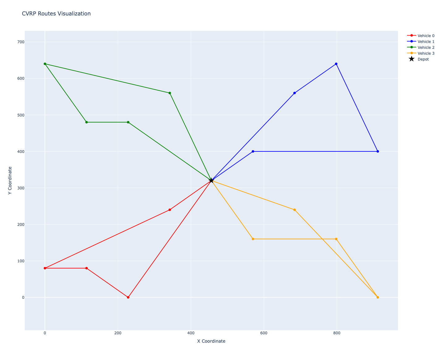
10. Visualize run assets
The Nextmv-ified main.py script contains a method called
create_route_visualization, which was created by us. This method uses
plotly to create a visualization for the given example: the routes assigned
to the vehicles, departing and returning to the depot. We are going to use the
location coordinates provided by the OR-Tools example
to visualize the routes.
Create a new input_with_coordinates.json file in the inputs directory which
includes the coordinates:
{
  "distance_matrix": [
    [
      0, 548, 776, 696, 582, 274, 502, 194, 308, 194, 536, 502, 388, 354, 468,
      776, 662
    ],
    [
      548, 0, 684, 308, 194, 502, 730, 354, 696, 742, 1084, 594, 480, 674, 1016,
      868, 1210
    ],
    [
      776, 684, 0, 992, 878, 502, 274, 810, 468, 742, 400, 1278, 1164, 1130,
      788, 1552, 754
    ],
    [
      696, 308, 992, 0, 114, 650, 878, 502, 844, 890, 1232, 514, 628, 822, 1164,
      560, 1358
    ],
    [
      582, 194, 878, 114, 0, 536, 764, 388, 730, 776, 1118, 400, 514, 708, 1050,
      674, 1244
    ],
    [
      274, 502, 502, 650, 536, 0, 228, 308, 194, 240, 582, 776, 662, 628, 514,
      1050, 708
    ],
    [
      502, 730, 274, 878, 764, 228, 0, 536, 194, 468, 354, 1004, 890, 856, 514,
      1278, 480
    ],
    [
      194, 354, 810, 502, 388, 308, 536, 0, 342, 388, 730, 468, 354, 320, 662,
      742, 856
    ],
    [
      308, 696, 468, 844, 730, 194, 194, 342, 0, 274, 388, 810, 696, 662, 320,
      1084, 514
    ],
    [
      194, 742, 742, 890, 776, 240, 468, 388, 274, 0, 342, 536, 422, 388, 274,
      810, 468
    ],
    [
      536, 1084, 400, 1232, 1118, 582, 354, 730, 388, 342, 0, 878, 764, 730,
      388, 1152, 354
    ],
    [
      502, 594, 1278, 514, 400, 776, 1004, 468, 810, 536, 878, 0, 114, 308, 650,
      274, 844
    ],
    [
      388, 480, 1164, 628, 514, 662, 890, 354, 696, 422, 764, 114, 0, 194, 536,
      388, 730
    ],
    [
      354, 674, 1130, 822, 708, 628, 856, 320, 662, 388, 730, 308, 194, 0, 342,
      422, 536
    ],
    [
      468, 1016, 788, 1164, 1050, 514, 514, 662, 320, 274, 388, 650, 536, 342,
      0, 764, 194
    ],
    [
      776, 868, 1552, 560, 674, 1050, 1278, 742, 1084, 810, 1152, 274, 388, 422,
      764, 0, 798
    ],
    [
      662, 1210, 754, 1358, 1244, 708, 480, 856, 514, 468, 354, 844, 730, 536,
      194, 798, 0
    ]
  ],
  "demands": [0, 1, 1, 2, 4, 2, 4, 8, 8, 1, 2, 1, 2, 4, 4, 8, 8],
  "vehicle_capacities": [15, 15, 15, 15],
  "num_vehicles": 4,
  "depot": 0,
  "coordinates": [
    [456, 320],
    [228, 0],
    [912, 0],
    [0, 80],
    [114, 80],
    [570, 160],
    [798, 160],
    [342, 240],
    [684, 240],
    [570, 400],
    [912, 400],
    [114, 480],
    [228, 480],
    [342, 560],
    [684, 560],
    [0, 640],
    [798, 640]
  ]
}
Up until now, the main.py script has not created any run assets given that no
coordinates were given. Now, we can run the app again using this new input
file to generate the visualization assets. You can use the nextmv local run
visuals command to visualize the assets of a run.
Execute the following command, which starts a new run, waits for it to complete, and visualizes the run's assets:
✅ Run local-y9r6vxxk created.
⏳ Getting run results...
💡 Removed assets from output for cleaner display, use --output to save the full output.
⏳ Getting run visuals...
✅ Run visuals opened in web browser, here are the local URLs of the visual files:
[
  "file:///user/free-local-experience/nextmv-ified/.nextmv/runs/local-y9r6vxxk/visuals/Routes_0.html"
]
The following libraries are supported for visualizing assets with the nextmv
local run visuals command:
plotlyfolium
This will also open a browser window for each asset produced by the run. You should see a simple plot like the following:
This command is saved as app5.sh in the full tutorial
code.
11. Understanding what happened
If you inspect the application directory consolidated in step 5 again, you will see a structure similar to the following:
.
├── .nextmv
│   └── runs
│       ├── {RUN_1}
│       │   ├── inputs
│       │   │   └── input.json
│       │   ├── {RUN_1}.json
│       │   ├── logs
│       │   │   └── logs.log
│       │   ├── outputs
│       │   │   ├── assets.json
│       │   │   ├── metrics.json
│       │   │   └── solutions
│       │   │       └── solution.json
│       │   └── visuals
│       ├── {RUN_2}
│       │   ├── inputs
│       │   │   └── input.json
│       │   ├── {RUN_2}.json
│       │   ├── logs
│       │   │   └── logs.log
│       │   ├── outputs
│       │   │   ├── assets.json
│       │   │   ├── metrics.json
│       │   │   └── solutions
│       │   │       └── solution.json
│       │   └── visuals
│       ├── {RUN_3}
│       │   ├── inputs
│       │   │   └── input.json
│       │   ├── {RUN_3}.json
│       │   ├── logs
│       │   │   └── logs.log
│       │   ├── outputs
│       │   │   ├── assets.json
│       │   │   ├── metrics.json
│       │   │   └── solutions
│       │   │       └── solution.json
│       │   └── visuals
│       └── {RUN_4}
│           ├── inputs
│           │   └── input.json
│           ├── {RUN_4}.json
│           ├── logs
│           │   └── logs.log
│           ├── outputs
│           │   ├── assets.json
│           │   ├── metrics.json
│           │   └── solutions
│           │       └── solution.json
│           └── visuals
│               └── Routes_0.html
├── app.yaml
├── inputs
│   ├── input_with_coordinates.json
│   └── input.json
├── main.py
├── pyproject.toml
└── uv.lock
The .nextmv dir is used to store and manage the local applications runs in
a structured way. The nextmv local command tree is used to interact with
these files, with methods for starting runs, retrieving results, visualizing
charts, and more.
🎉🎉🎉 Congratulations, you have finished this tutorial!
Full tutorial code
You can find the consolidated code examples used in this tutorial in the
tutorials GitHub repository. The
free-local-experience dir contains all the
code that was shown in this tutorial.
For the example, you will find two directories:
original: the original example without any modifications.nextmv-ified: the example converted into a Nextmv application.
Go into each directory for instructions about running the decision model.